R PROGRAMMING HELP

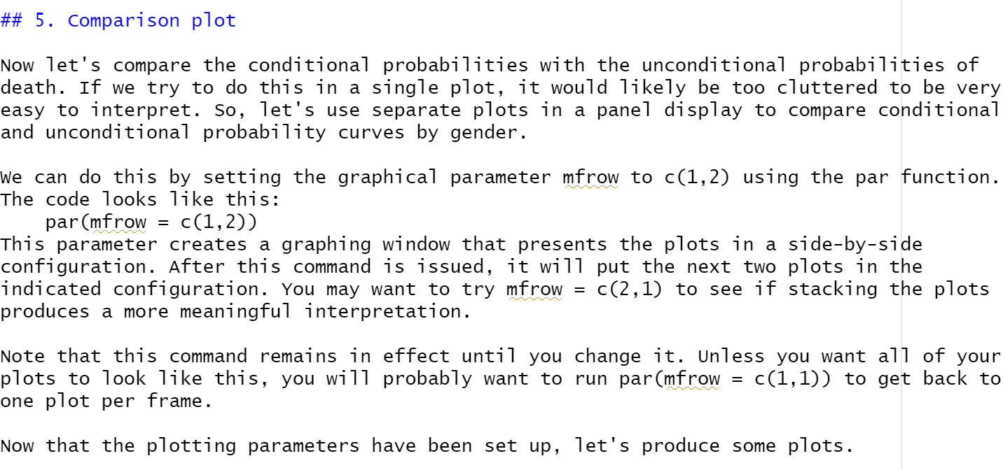
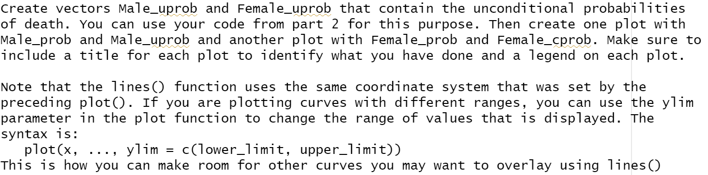
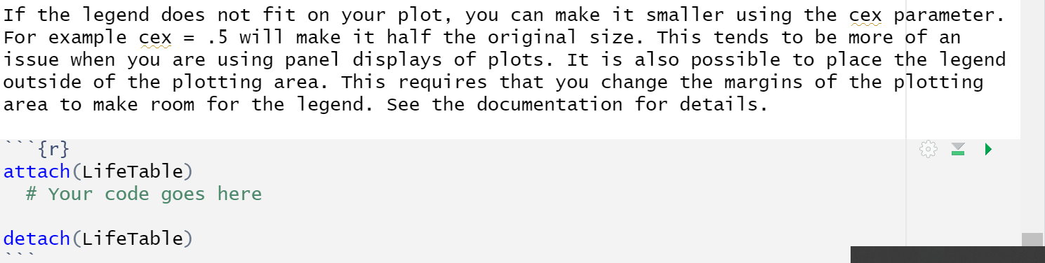
## 5. Comparison plot Now let's compare the conditional probabilities with the unconditional probabilities of death. If we try to do this in a single plot, it would likely be too cluttered to be very easy to interpret. So, let's use separate plots in a panel display to compare conditional and unconditional probability curves by gender. = We can do this by setting the graphical parameter mfrow to c(1,2) using the par function. The code looks like this: par(mfrow = C(1,2)) This parameter creates a graphing window that presents the plots in a side-by-side configuration. After this command is issued, it will put the next two plots in the indicated configuration. You may want to try mfrow C(2,1) to see if stacking the plots produces a more meaningful interpretation. = Note that this command remains in effect until you change it. Unless you want all of your plots to look like this, you will probably want to run par(mfrow C(1,1)) to get back to one plot per frame. = Now that the plotting parameters have been set up, let's produce some plots. Create vectors Male_uprob and Female_uprob that contain the unconditional probabilities of death. You can use your code from part for this purpose. Then create one plot with Male_prob and Male_uprob and another plot with Female_prob and Female_cprob. Make sure to include a title for each plot to identify what you have done and a legend on each plot. Note that the lines () function uses the same coordinate system that was set by the preceding plot(). If you are plotting curves with different ranges, you can use the ylim parameter in the plot function to change the range of values that is displayed. The syntax is: plot(x, ylim = c(lower_limit, upper_limit)) This is how you can make room for other curves you may want to overlay using lines () If the legend does not fit on your plot, you can make it smaller using the cex parameter. For example cex = .5 will make it half the original size. This tends to be more of an issue when you are using panel displays of plots. It is also possible to place the legend outside of the plotting area. This requires that you change the margins of the plotting area to make room for the legend. See the documentation for details. {r} attach(LifeTable) # Your code goes here detach (LifeTable)