R PROGRAMMING. PLEASE HELP ME FIX THE PLOT. IDK WHY THE LEGEND ISNT SHOWING UP.

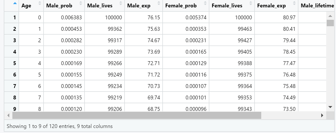
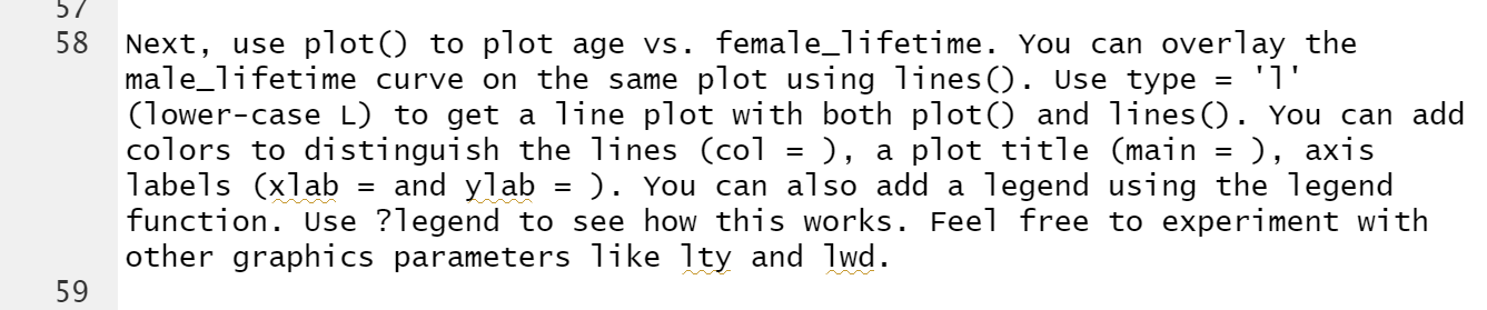
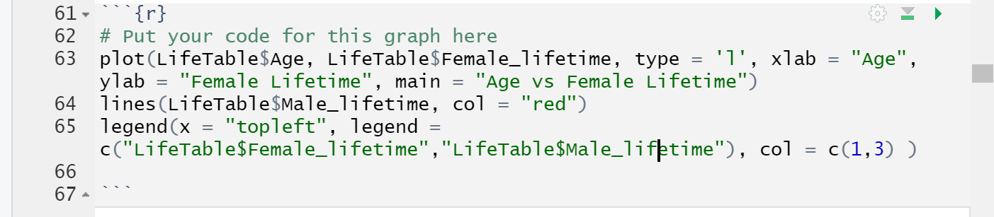
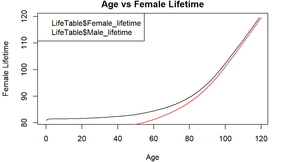
Age Male_prob Male_lives Male_exp Female_prob Female lives Female_exp Male lifetime 1 0 0.006383 100000 76.15 0.005374 100000 80.97 2 1 0.000453 99362 75.63 0.000353 99463 80.41 3 2 0.000282 99317 74.67 0.000231 99427 79.44 4 3 0.000230 99289 73.69 0.000165 99405 78.45 5 4 0.000169 99266 72.71 0.000129 99388 77.47 6 5 0.000155 99249 71.72 0.000116 99375 76.48 7 6 0.000145 99234 70.73 0.000107 99364 75.48 8 00 7 0.000135 99219 69.74 0.000101 99353 74.49 9 8 0.000120 99206 68.75 0.000096 99343 73.50 Showing 1 to 9 of 120 entries, 9 total columns 57 58 Next, use plot() to plot age vs. female_lifetime. You can overlay the male_lifetime curve on the same plot using lines (). Use type = 'l' (lower-case L) to get a line plot with both plot() and lines (). You can add colors to distinguish the lines (col = ), a plot title (main ), axis labels (xlab = and ylab = ). You can also add a legend using the legend function. Use ?legend to see how this works. Feel free to experiment with other graphics parameters like Ity and lwd. = = = 59 = - = 61 '{r} 62 # Put your code for this graph here 63 plot(LifeTable$Age, LifeTable$Female_lifetime, type l', xlab "Age", ylab = "Female Lifetime", main = "Age vs Female Lifetime") 64 lines(LifeTable$Male_lifetime, col "red") 65 legend (x = "topleft", legend c("LifeTable$Female_lifetime","lifeTable $Male_lifetime"), col = c(1,3) ) 66 67 - - Age vs Female Lifetime 120 LifeTable$Female_lifetime LifeTable$Male_lifetime 110 Female Lifetime 100 90 80 0 20 40 60 80 100 120 Age 68 - 69 ### Question 2: what do you observe about differences in expected lifetimes between males and females? 70 Age Male_prob Male_lives Male_exp Female_prob Female lives Female_exp Male lifetime 1 0 0.006383 100000 76.15 0.005374 100000 80.97 2 1 0.000453 99362 75.63 0.000353 99463 80.41 3 2 0.000282 99317 74.67 0.000231 99427 79.44 4 3 0.000230 99289 73.69 0.000165 99405 78.45 5 4 0.000169 99266 72.71 0.000129 99388 77.47 6 5 0.000155 99249 71.72 0.000116 99375 76.48 7 6 0.000145 99234 70.73 0.000107 99364 75.48 8 00 7 0.000135 99219 69.74 0.000101 99353 74.49 9 8 0.000120 99206 68.75 0.000096 99343 73.50 Showing 1 to 9 of 120 entries, 9 total columns 57 58 Next, use plot() to plot age vs. female_lifetime. You can overlay the male_lifetime curve on the same plot using lines (). Use type = 'l' (lower-case L) to get a line plot with both plot() and lines (). You can add colors to distinguish the lines (col = ), a plot title (main ), axis labels (xlab = and ylab = ). You can also add a legend using the legend function. Use ?legend to see how this works. Feel free to experiment with other graphics parameters like Ity and lwd. = = = 59 = - = 61 '{r} 62 # Put your code for this graph here 63 plot(LifeTable$Age, LifeTable$Female_lifetime, type l', xlab "Age", ylab = "Female Lifetime", main = "Age vs Female Lifetime") 64 lines(LifeTable$Male_lifetime, col "red") 65 legend (x = "topleft", legend c("LifeTable$Female_lifetime","lifeTable $Male_lifetime"), col = c(1,3) ) 66 67 - - Age vs Female Lifetime 120 LifeTable$Female_lifetime LifeTable$Male_lifetime 110 Female Lifetime 100 90 80 0 20 40 60 80 100 120 Age 68 - 69 ### Question 2: what do you observe about differences in expected lifetimes between males and females? 70