Regression Result #1:

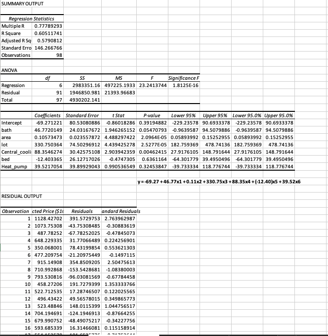
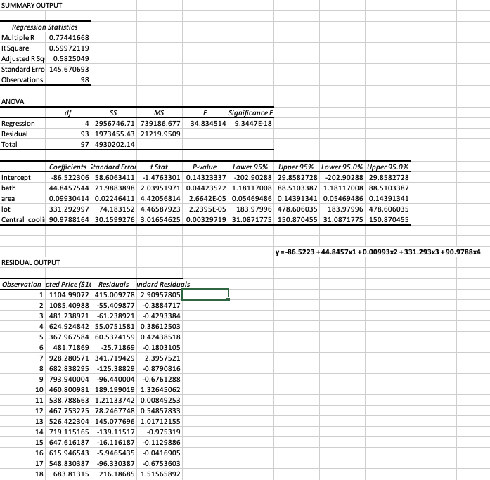
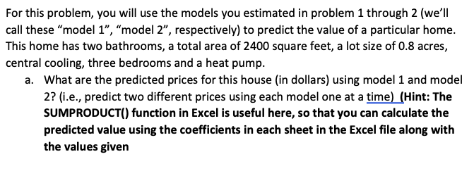
SUMMARY OUTPUT Regression Statistics Multiple R 0.77789293 Square 0.60511741 Adjusted R 5q 0.5790812 Standard Erro 146.266766 Observations 98 ANOVA of SS MS F Significance F Regression 6 2983351.16 497225.1933 23.2413744 1.8125E-16 Residual 91 1946850.981 21393.96683 Tota 97 4930202.141 Coefficients Standard Error : Stat P-value Lower 95% Upper 95%% Lower 95.0% Upper 95.0% Intercept 69.271221 80.53080886 -0.86018286 0.39194882 -229.23578 90.6933378 -229.23578 90.6933378 bath 46.7720149 24.03167672 1.946265152 0.05470793 -0.9639587 94.5079886 -0.9639587 94.5079886 area 0.10573473 0.023557872 4.488297422 2.0964E-05 0.05893992 0.15252955 0.05893992 0.15252955 lot 330.750364 74.50296912 4.439425278 2.52776-05 182.759369 478.74136 182.759369 478.74136 Central_cooli 88.3546274 30.42575108 2.903942359 0.00462415 27.9176105 148.791644 27.9176105 148.791644 bed -12.403365 26.12717026 -0.4747305 0.6361164 -64.301779 39.4950496 -64.301779 39.4950496 Heat_pump 39.5217054 39.89929043 0.990536549 0.32453847 -39.733334 118.776744 -39.733334 118.776744 y=-69.27+46.77x1 +0.11x2 +330.75x3 +88.35x4 + (-12.40)x5 +39.52x6 RESIDUAL OUTPUT Observation c Residuals andard Residuals 1 1128.42702 391.5729753 2.763962987 2 1073.75308 -43.75308485 -0.30883619 487.78252 -67.78252025 -0.47845073 4 648.229335 31.77066489 0.224256901 5 350.068001 78.43199854 0.553621303 6 477.209754 -21.20975449 -0.1497115 7 915.14908 354.8509205 2.50475613 8 710.992868 -153.5428681 -1.08380003 9 793.530816 -96.03081569 -0.67784458 10 458.27206 191.7279399 1.353333766 11 522.712535 17.28746507 0.122025565 12 496.43422 49.56578015 0.349865773 13 523.48846 148.0115399 1.044756517 14 704.194691 -124.1946913 -0.87664255 15 679.990752 -48.49075217 -0.34227756 16 593.685339 16.31466081 0.115158914SUMMARY OUTPUT Regression Statistics Multiple R 0.77441668 R Square 0.59972119 Adjusted R Sq 0.5825049 Standard Erro 145.670693 Observations 98 ANOVA $5 MS F Significance F Regression 4 2956746.71 739186.677 34.834514 9.3447E-18 Residual 93 1973455.43 21219.9509 Tota 97 4930202.14 Coefficients itandard Error t Stat P-value Lower 95% Upper 95%% Lower 95.0% Upper 95.0% Intercept 86.522306 58.6063411 -1.4763301 0.14323337 -202.90288 29.8582728 -202.90288 29.8582728 bath 44.8457544 21.9883898 2.03951971 0.04423522 1.18117008 88.5103387 1.18117008 88.5103387 area 0.09930414 0.02246411 4.42056814 2.6642E-05 0.05469486 0.14391341 0.05469486 0.14391341 lot 331.292997 74.183152 4.46587923 2.2395E-05 183.97996 478.606035 183.97996 478.606035 Central_cooli 90.9788164 30.1599276 3.01654625 0.00329719 31.0871775 150.870455 31.0871775 150.870455 y=-86.5223 +44.8457x1 +0.00993x2 +331.293x3 +90.9788x4 RESIDUAL OUTPUT Observation cted Price ($10 Residuals indard Residuals 1 1104.99072 415.009278 2.90957805 2 1085.40988 -55.409877 -0.3884717 3 481.238921 -61.238921 -0.4293384 4 624.924842 55.0751581 0.38612503 5 367.967584 60.5324159 0.42438518 6 481.71869 -25.71869 -0.1803105 7 928.280571 341.719429 2.3957521 8 682.838295 -125.38829 0.8790816 9 793.940004 -96.440004 -0.6761288 10 460.800981 189.199019 1.32645062 11 538.788663 1.21133742 0.00849253 12 467.753225 78.2467748 0.54857833 13 526.422304 145.077696 1.01712155 14 719.115165 -139.11517 -0.975319 15 647.616187 -16.116187 -0.1129886 16 615.946543 -5.9465435 -0.0416905 17 548.830387 -96.330387 -0.6753603 18 683.81315 216.18685 1.51565892For this problem, you will use the models you estimated in problem 1 through 2 (we'll call these "model 1", "model 2", respectively) to predict the value of a particular home. This home has two bathrooms, a total area of 2400 square feet, a lot size of 0.8 acres, central cooling, three bedrooms and a heat pump. a. What are the predicted prices for this house (in dollars) using model 1 and model 2? (i.e., predict two different prices using each model one at a time) (Hint: The SUMPRODUCT() function in Excel is useful here, so that you can calculate the predicted value using the coefficients in each sheet in the Excel file along with the values given