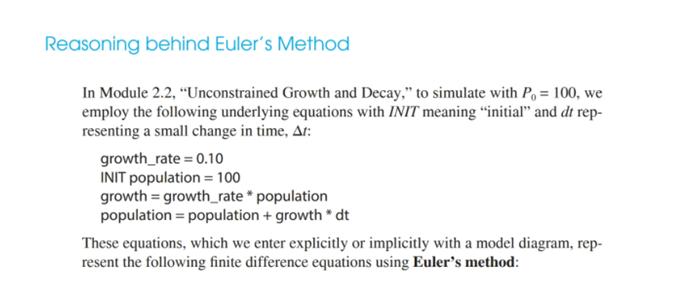
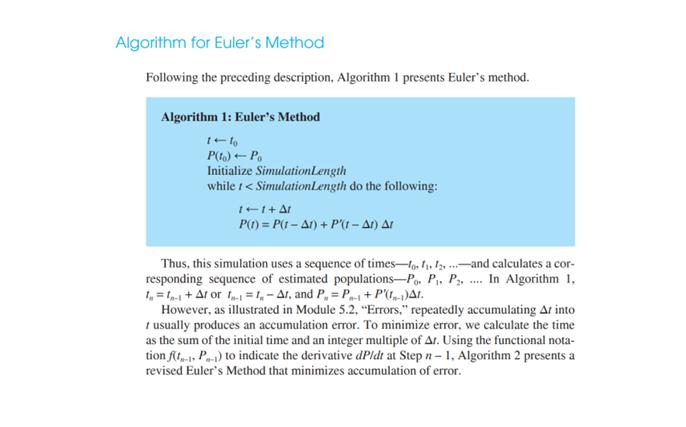
Repeat the exercises of Module 6.2, "Euler's Method," using the Runge-Kutta 4 method. Compare the relative errors with those of the corresponding exercises from Module 6.2, "Euler's Method," and Module 6.3, "Runge-Kutta 2 Method." 6. Download the file simplePendulum from the text's website in one of the sys- tem dynamics tools. Figure 3.3.3 of Module 3.3, "Tick Tock-The Pendu- lum Clock," shows a plot of a simple pendulum's angle, angular velocity, and angular acceleration versus time that is the result of the simulation with At = 0.01 and Runga-Kutta 4 integration. Run the simulation with At = 0.01 using, in turn, Runga-Kutta 4, Runga-Kutta 2, and Euler's methods or what- ever methods are available with your system dynamics tool. Describe any anomalies in the graphs. Repeat the simulations and description for At = 0.1. Discuss the implications of your findings. Reasoning behind Euler's Method In Module 2.2, "Unconstrained Growth and Decay," to simulate with P,= 100, we employ the following underlying equations with INIT meaning "initial" and dt rep- resenting a small change in time, Ar: growth_rate= 0.10 INIT population = 100 growth = growth_rate * population population = population + growth * dt These equations, which we enter explicitly or implicitly with a model diagram, rep- resent the following finite difference equations using Euler's method: growth_rate=U.IU population (0) 100 growth(t) = growth_rate* population(t-At) population (t) = population (t - At) + growth(t) * At The population at one time step, population (1), is the population at the previous time step, population (t-Ar), plus the estimated change in population, growth(t) * Ar. The derivative of population with respect to time is growth, and growth(t) = growth_rate * population(t - At) = 0.10 * population (1 - At) or dPldt = 0.10P. The change in the population is the flow (in this case, growth) times the change in time, Ar; and the flow (growth) is the derivative of the function at the previous time step, t-At. Figure 6.2.1 illustrates Euler's method used to estimate P = P(8) for the preced- ing differential equation by starting with P, = P(0) = 100 and using At = 8. In this situation, t = 8,1- Ar=0, and the derivative at that time is P'(0) = 0.1(100) = 10, which, as Figure 6.2.1 depicts, is the slope of the tangent line to the curve P(t) at (0. 100). We multiply Ar, 8, by this derivative at the previous time step, 10, to obtain the estimated change in P, 80. Consequently, the estimate for P, is as follows: estimate for P = previous value of P + estimated change in P = P+ P'(0)Ar = 100 + 10(8) = 180 In Module 2.2, "Unconstrained Growth and Decay," we discovered analytically that the solution to the preceding differential equation is P = 100e. Because the graph of the actual function is concave up, this estimated value, 180, is lower than the ac- tual value at t = 8, 100 223. 300 250 200 150 100 50 (8, 223) 4 (8, 180) 80 6 100 4 -2 8 10 12 Figure 6.2.1 Actual point, (8, 223), and point obtained by Euler's method, (8, 180) I [ Algorithm for Euler's Method Following the preceding description, Algorithm 1 presents Euler's method. Algorithm 1: Euler's Method P(to) -Po Initialize SimulationLength while 1 < SimulationLength do the following: 1+1+ Ar P(1)=P(1-A1) + P'(r-Ar) Ar Thus, this simulation uses a sequence of times-1.12-and calculates a cor- responding sequence of estimated populations-Po. P, P,... In Algorithm 1, 1 =1-1+Af or 1-1=1,- Ar, and P, = P + P()AL. However, as illustrated in Module 5.2, "Errors," repeatedly accumulating Ar into I usually produces an accumulation error. To minimize error, we calculate the time as the sum of the initial time and an integer multiple of Ar. Using the functional nota- tion ft. P-1) to indicate the derivative dPldt at Step n-1, Algorithm 2 presents a revised Euler's Method that minimizes accumulation of error.