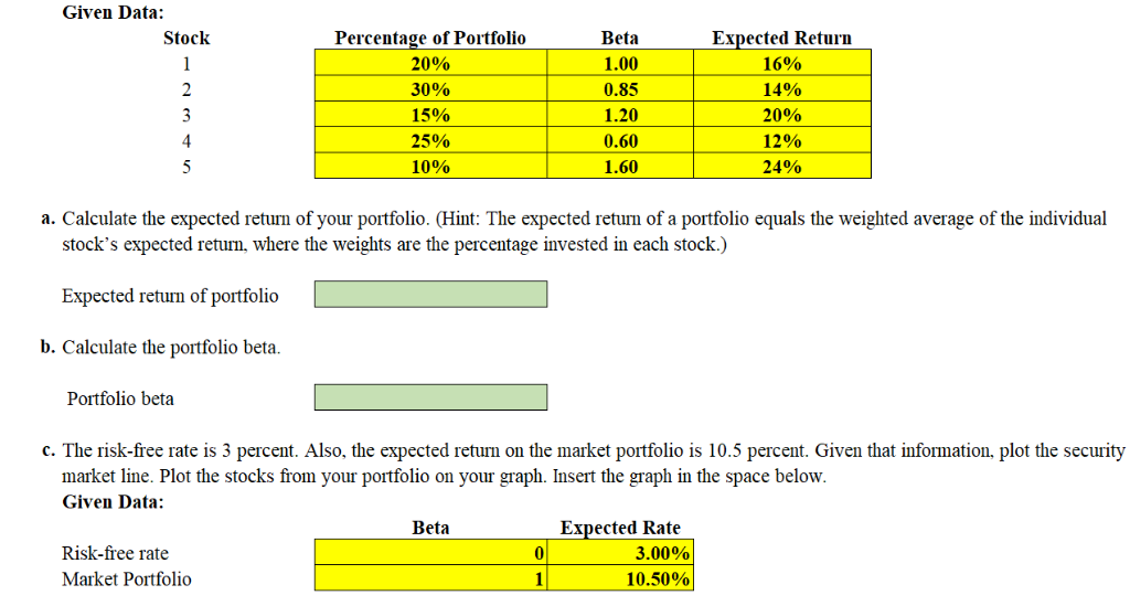
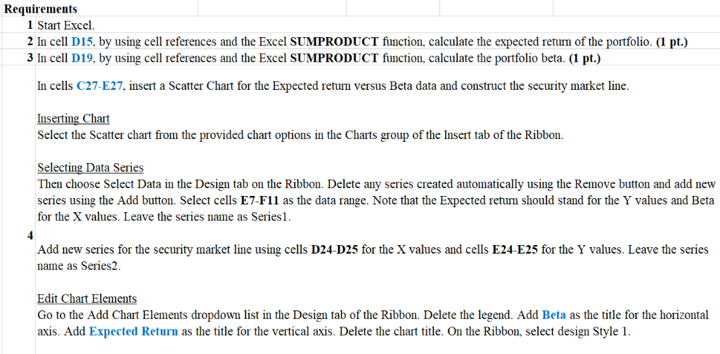
Requirements 1 Start Excel. 2 In cell D15, by using cell references and the Excel SUMPRODUCT function, calculate the expected retum of the portfolio. (1 pt.) 3 In cell D19, by using cell references and the Excel SUMPRODUCT function, calculate the portfolio beta. (1 pt.) In cells C27-E27, insert a Scatter Chart for the Expected returm versus Beta data and construct the security market line. Inserting Chart Select the Scatter chart from the provided chart options in the Charts group of the Insert tab of the Ribbon. Selecting Data Series Then choose Select Data in the Design tab on the Ribbon. Delete any series created automatically using the Remove button and add new series using the Add button. Select cells E7-F1l as the data range. Note that the Expected retun should stand for the Y values and Beta for the X values. Leave the series name as Series1. Add new series for the security market line using cells D24-D25 for the X values and cells E24-E25 for the Y values. Leave the series name as Series2 lidie Cbari Elemnnis Go to the Add Chart Elements dropdown list in the Design tab of the Ribbon. Delete the legend. Add Beta as the title for the horizontal axis. Add Expected Return as the title for the vertical axis. Delete the chart title. On the Ribbon, select design Style 1. Requirements 1 Start Excel. 2 In cell D15, by using cell references and the Excel SUMPRODUCT function, calculate the expected retum of the portfolio. (1 pt.) 3 In cell D19, by using cell references and the Excel SUMPRODUCT function, calculate the portfolio beta. (1 pt.) In cells C27-E27, insert a Scatter Chart for the Expected returm versus Beta data and construct the security market line. Inserting Chart Select the Scatter chart from the provided chart options in the Charts group of the Insert tab of the Ribbon. Selecting Data Series Then choose Select Data in the Design tab on the Ribbon. Delete any series created automatically using the Remove button and add new series using the Add button. Select cells E7-F1l as the data range. Note that the Expected retun should stand for the Y values and Beta for the X values. Leave the series name as Series1. Add new series for the security market line using cells D24-D25 for the X values and cells E24-E25 for the Y values. Leave the series name as Series2 lidie Cbari Elemnnis Go to the Add Chart Elements dropdown list in the Design tab of the Ribbon. Delete the legend. Add Beta as the title for the horizontal axis. Add Expected Return as the title for the vertical axis. Delete the chart title. On the Ribbon, select design Style 1