Sample :

---------------- matlab program file ode02.m ------------------------

% The first part of this m-file the matlab function ode45 to solve

% the first order ode dy/dt = f(t,y) for t0

% where f(t,y) is the function defined by the m-file ode01f.m,

% under the initial condition y = y0 at t = t0, and plot the solution curve.

% This is the same ode solved in project 1 using Euler approximation.

% The second part solves the second order ode y" + ty' + cos(t)y = t sin(t),

% for t_0

% and plots the solution and its derivative.

% Regarding y as a vector valued function with two components y1 and y2,

% where y1 is the solution itself and y2 its derivative,

% the equation may be written as a system of two equations:

% y1' = y2 and y2' = t sin(t) - cos(t) y1 - t y2

% with initial condition y1(0) = y0 and y2(0) = yp0.

% The two equations may be written as a single equation in vector form:

% y' = f(t,y),

% where y1

% f(t,y) = ( )

% t sin(t) - cos(t) y1 - t y2

% is a vector valued function defined by m-file ode02f.m.

% start of part 1 (initializing constants)

clear; t0 = 0; t1 = 2*pi; y0 = 1.5;

% apply ode45 to get t values and y values

[t y] = ode45('ode01f', [t0 t1], y0);

% plot solution curve

plot(t, y);

title('Solution curve of the first order ode');

xlabel('Time t');

ylabel('y values');

'press any key to continue'

pause;

% calculate the solution at t = 2

t1 = 2;

[t y] = ode45('ode01f', [t0 t1], y0);

s=size(y); n=s(1);

'value of the solution of the 1st order at t = 2 is '

y(n) % compare this with the value obtained in project 1

'press any key to continue'

pause;

% start of part 2 (initializing constants)

clear; t0 = 0; t1 = 5; y0 = 2; yp0 = -3;

% Apply ode45 to get time t values and solution y values, where

% where y is a matrix with two columns, y(:,1) is the first column

% containing the solution values y1 and y(:,2) is the second column

% containing the values of its derivatives y2.

[t y] = ode45('ode02f', [t0 t1], [y0 yp0]);

% Plot the solution curve and its derivative

plot(t, y(:,1));

title('Solution curve and its derivative of the 2nd order ode');

xlabel('Time t');

ylabel('y and y prime values');

hold on;

plot(t, y(:,2));

hold off;

------------------- matlab function file ode02f.m ------------------

% The vector valued function defined in this m-file

% is used to solve the second order equation

% y" + ty' + cos(t)y = t sin(t).

function fun = f(t,y)

fun(1)=y(2);

fun(2)=t*sin(t)-cos(t)*y(1)-t*y(2);

fun=fun'; % convert a row vector (1X2 matrix) to a column vector (2X1 matrix

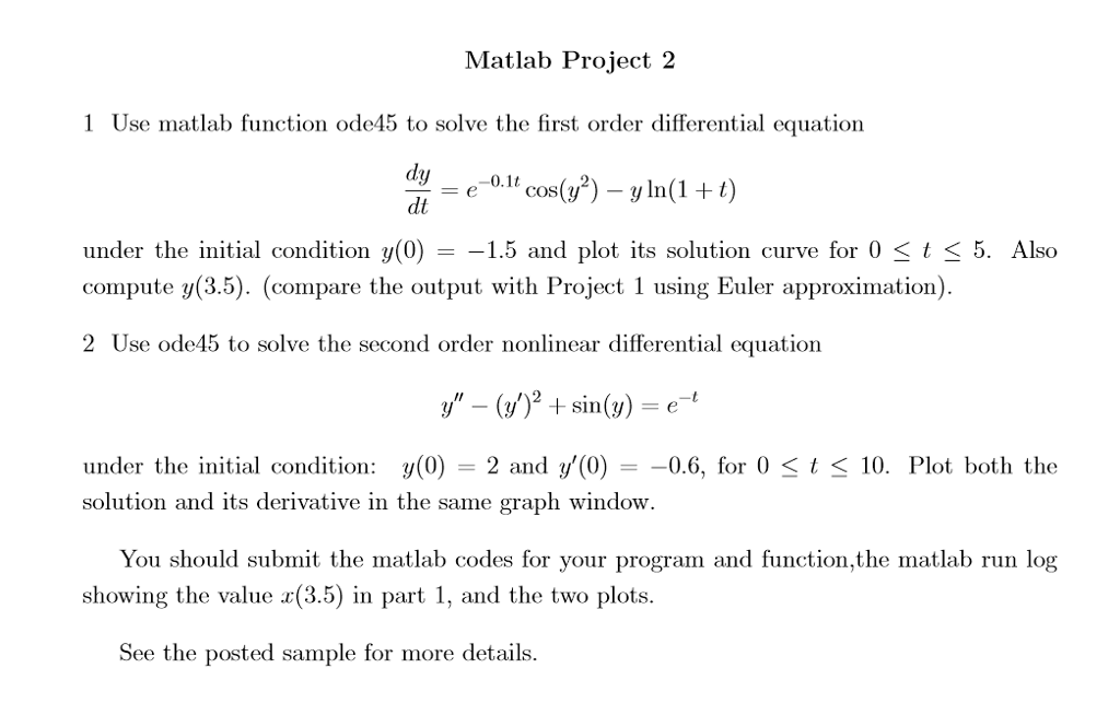
Matlab Project 2 1 Use matlab function ode45 to solve the first order differential equation dy 0.1t cos(y) y ln (1 t) dt under the initial condition y(0) 1.5 and plot its solution curve for 0 s t S 5. Also compute y 3.5). (compare the output with Project 1 using Euler approximation). 2 Use ode45 to solve the second order nonlinear differential equation under the initial condition y(0) 2 and y' (0) 0.6, for 0 S t S 10. Plot both the solution and its derivative in the same graph window You should submit the matlab codes for your program and function,the matlab run log showing the value (3.5 in part 1, and the two plots. See the posted sample for more details