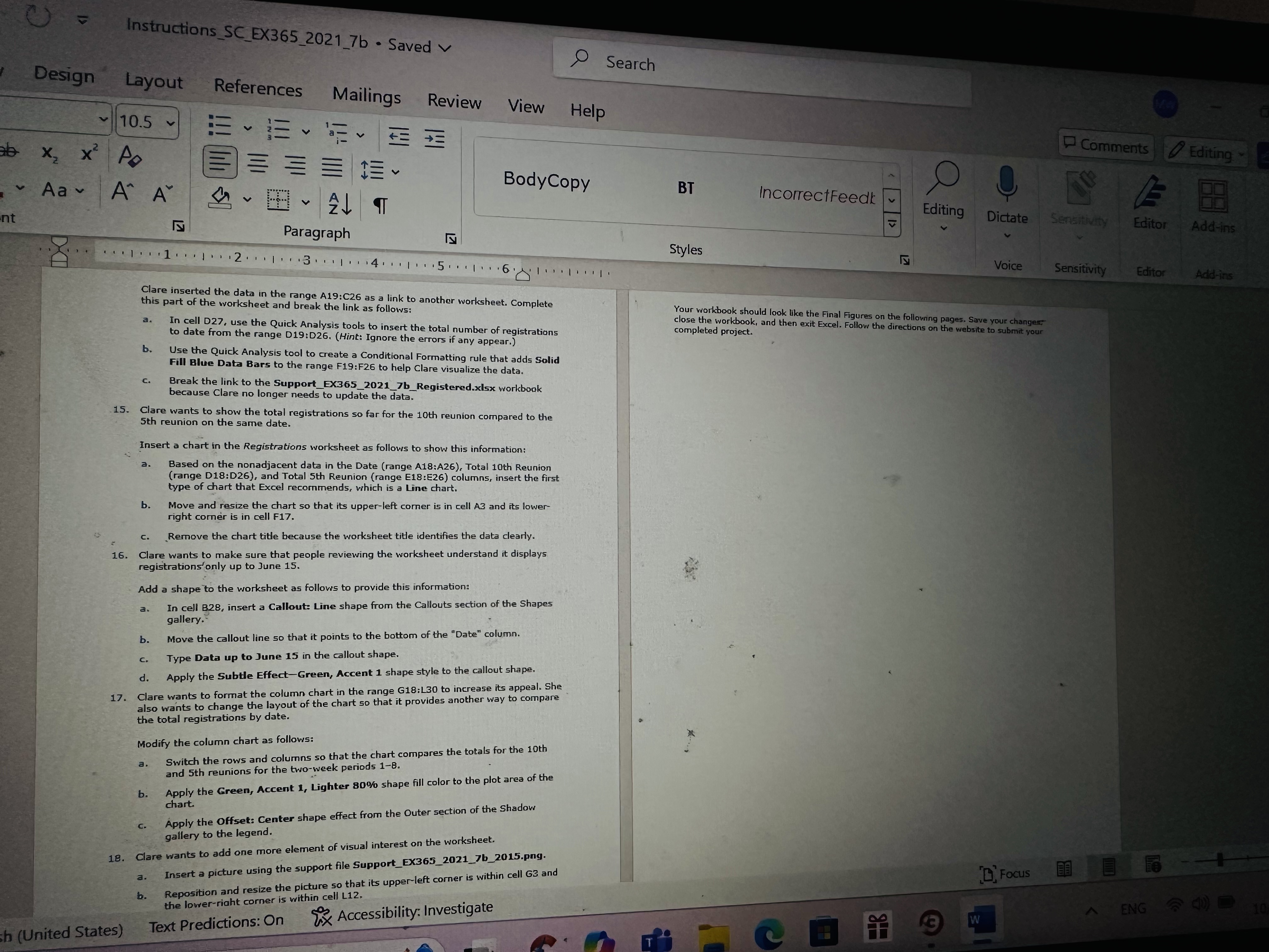
$$

Search

Design Layout References Mailings Review View Help

Comments

Editing

Clare inserted the data in the range A$19$:C$26$ as a link to another worksheet. Complete

this part of the worksheet and break the link as follows:

a$.$ In cell D$27,$ use the Quick Analysis tools to insert the total number of registrations to date from the range D$19$:D$26.($Hint: Ignore the errors if any appear.$)$

b$.$ Use the Quick Analysis tool to create a Conditional Formatting rule that adds Solid Fill Blue Data Bars to the range F$19$:F$26$ to help Clare visualize the data.

c$.$ Break the link to the Support$\_$EX$365\_2021\_7$b$\_$Registered.xdsx workbook because Clare no longer needs to update the data.

$15.$ Clare wants to show the total registrations so far for the $10$th reunion compared to the $5$ th reunion on the same date.

Insert a chart in the Registrations worksheet as follows to show this information:

a$.$ Based on the nonadjacent data in the Date $($range A$18$:A$26),$ Total $10$th Reunion $($range D$18$:D$26),$ and Total $5$th Reunion $($range E$18$:E$26)$ columns, insert the first type of chart that Excel recommends, which is a Line chart.

b$.$ Move and resize the chart so that its upper$-$left comer is in cell A$3$ and its lower right comer is in cell F$17.$

c$.$ Remove the chart title because the worksheet title identifies the data clearly.

$16.$ Clare wants to make sure that people reviewing the worksheet understand it displays registrations' only up to June $15.$

Add a shape to the worksheet as follows to provide this information:

a$.$ In cell B$28,$ insert a Callout: Line shape from the Callouts section of the Shapes gallery.

b$.$ Move the callout line so that it points to the bottom of the "Date" column.

c$.$ Type Data up to June $15$ in the callout shape.

d$.$ Apply the Subtle Effect$-$Green, Accent $1$ shape style to the callout shape.

$17.$ Clare wants to format the column chart in the range G$18$:L$30$ to increase its appeal. She also wants to change the layout of the chart so that it provides another sway to compare the total registrations by date.

Modify the column chart as follows:

a$.$ Switch the rows and columns so that the chart compares the totals for the $10$ th and $5$ th reunions for the two$-$week periods $1-8.$

b$.$ Apply the Green, Accent $1,$ Lighter $80\%$ shape fill color to the plot area of the chart.

c$.$ Apply the Offset: Center shape effect from the Outer section of the Shadow gallery to the legend.

$18.$ Clare wants to add one more element of visual interest on the worksheet.

a$.$ Insert a picture using the support file Support$\_$EX$365\_2021\_7$b$\_2015.$png$.$

Your workbook should look like the Final Figures on the following pages. Save your changers close the workbook, and then exit Excel. Follow, the directions on the website to submit your completed project.

$$

Search

Design Layout References Mailings Review View Help

Comments

Editing

Clare inserted the data in the range A$19$:C$26$ as a link to another worksheet. Complete

this part of the worksheet and break the link as follows:

a$.$ In cell D$27,$ use the Quick Analysis tools to insert the total number of registrations to date from the range D$19$:D$26.($Hint: Ignore the errors if any appear.$)$

b$.$ Use the Quick Analysis tool to create a Conditional Formatting rule that adds Solid Fill Blue Data Bars to the range F$19$:F$26$ to help Clare visualize the data.

c$.$ Break the link to the Support$\_$EX$365\_2021\_7$b$\_$Registered.xdsx workbook because Clare no longer needs to update the data.

$15.$ Clare wants to show the total registrations so far for the $10$th reunion compared to the $5$ th reunion on the same date.

Insert a chart in the Registrations worksheet as follows to show this information:

a$.$ Based on the nonadjacent data in the Date $($range A$18$:A$26),$ Total $10$th Reunion $($range D$18$:D$26),$ and Total $5$th Reunion $($range E$18$:E$26)$ columns, insert the first type of chart that Excel recommends, which is a Line chart.

b$.$ Move and resize the chart so that its upper$-$left comer is in cell A$3$ and its lower right comer is in cell F$17.$

c$.$ Remove the chart title because the worksheet title identifies the data clearly.

$16.$ Clare wants to make sure that people reviewing the worksheet understand it displays registrations' only up to June $15.$

Add a shape to the worksheet as follows to provide this information:

a$.$ In cell B$28,$ insert a Callout: Line shape from the Callouts section of the Shapes gallery.

b$.$ Move the callout line so that it points to the bottom of the "Date" column.

c$.$ Type Data up to June $15$ in the callout shape.

d$.$ Apply the Subtle Effect$-$Green, Accent $1$ shape style to the callout shape.

$17.$ Clare wants to format the column chart in the range G$18$:L$30$ to increase its appeal. She also wants to change the layout of the chart so that it provides another sway to compare the total registrations by date.

Modify the column chart as follows:

a$.$ Switch the rows and columns so that the chart compares the totals for the $10$ th and $5$ th reunions for the two$-$week periods $1-8.$

b$.$ Apply the Green, Accent $1,$ Lighter $80\%$ shape fil