SISO system, find if the system is controllable (for control experts)

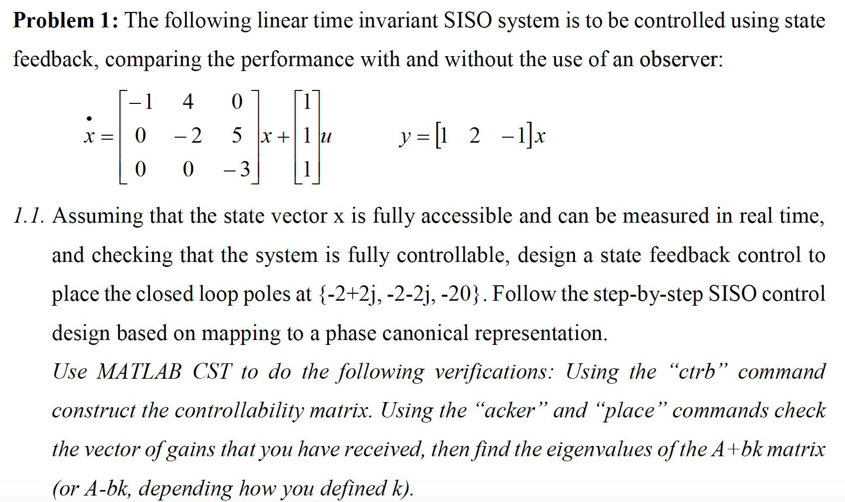
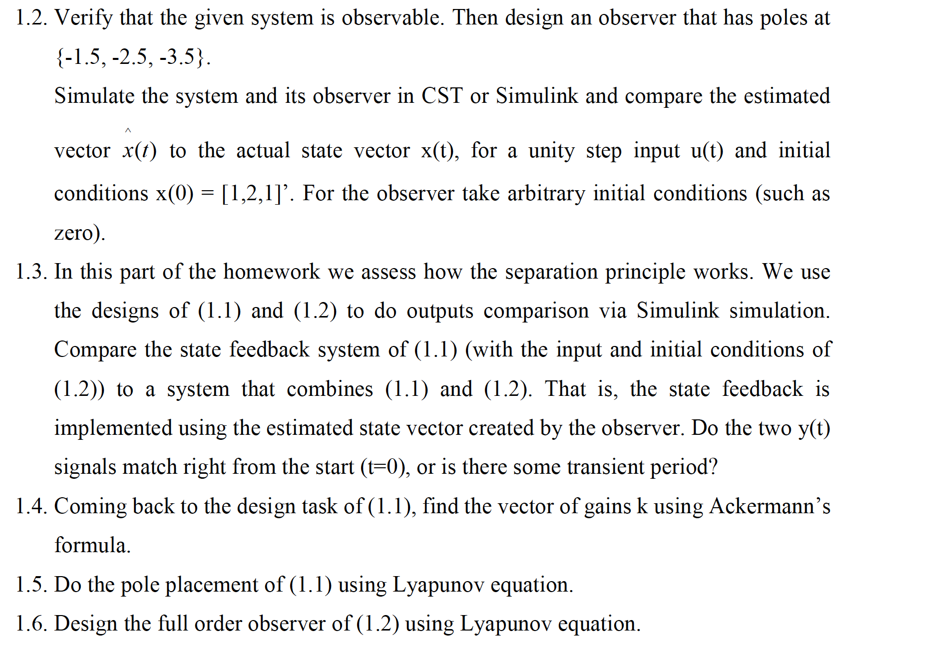
Problem 1: The following linear time invariant 8180 system is to be controlled using state feedback, comparing the performance with and without the use of an observer: 1 4 0 1 5c: 0 2 5 x+lu y=[1 2 l]x 0 0 3 l 1.]. Assuming that the state vector x is fully accessible and can be measured in real time, and checking that the system is fully controllable, design a state feedback control to place the closed loop poles at {-2+2j, -2-2j, -20}. Follow the step-by-step SISO control design based on mapping to a phase canonical representation. Use MAT LAB CST to do the following verications: Using the \"ctrb \" command construct the controllability matrix. Using the \"acker\" and \"place\" commands check the vector of gains that you have received, then find the eigenvalues of the A +bk matrix (or A-bk, depending how you defined k). 1.2. Verify that the given system is observable. Then design an observer that has poles at {-15, -2.5, -3.5}. Simulate the system and its observer in CST or Simulink and compare the estimated /\\ vector x(t) to the actual state vector x(t), for a unity step input u(t) and initial conditions x(0) = [1,2,1]'. For the observer take arbitrary initial conditions (such as zero). 1.3. In this part of the homework we assess how the separation principle works. We use the designs of (1 .1) and (1.2) to do outputs comparison via Simulink simulation. Compare the state feedback system of (1.1) (with the input and initial conditions of (1.2)) to a system that combines (1 .1) and (1.2). That is, the state feedback is implemented using the estimated state vector created by the observer. Do the two y(t) signals match right from the start (t=0), or is there some transient period? 1.4. Coming back to the design task of (1. 1), find the vector of gains k using Ackermann's formula. 1.5. Do the pole placement of (1.1) using Lyapunov equation. 1.6. Design the full order observer of (1.2) using Lyapunov equation