someone please help me with this project by step by step explaining.

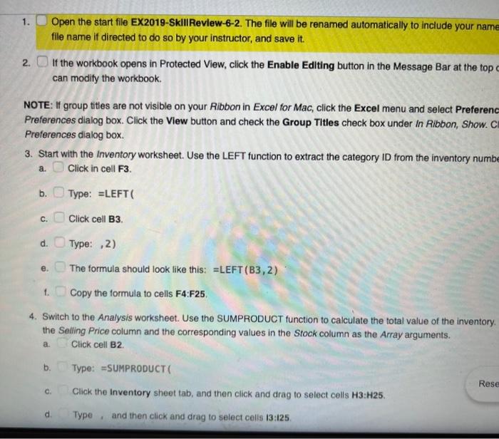
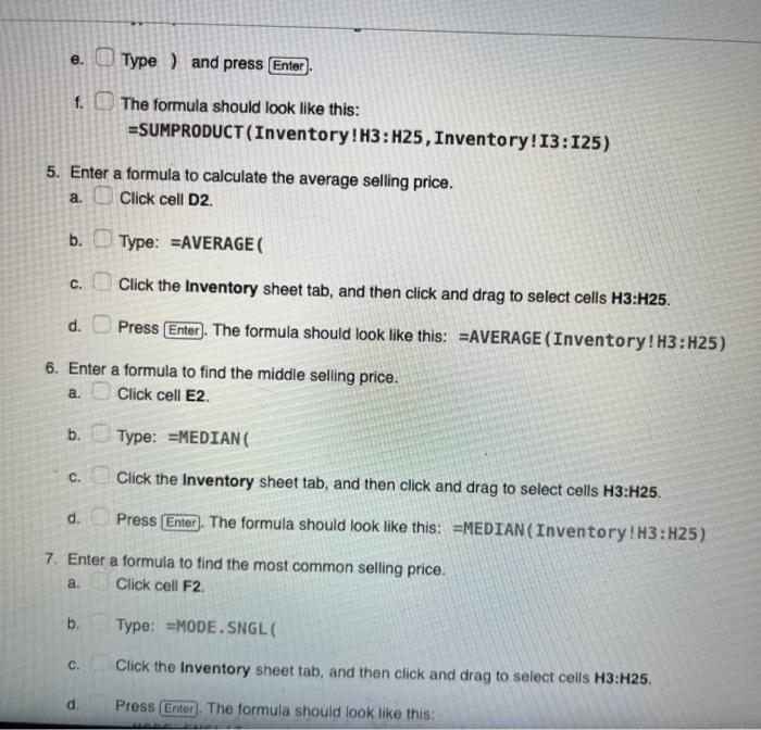
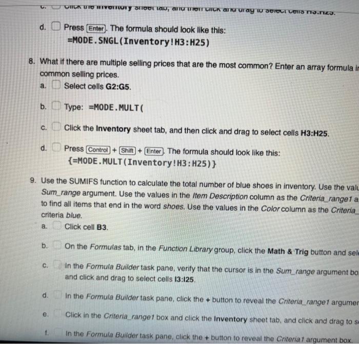
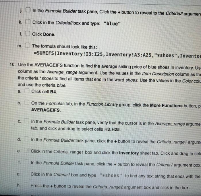
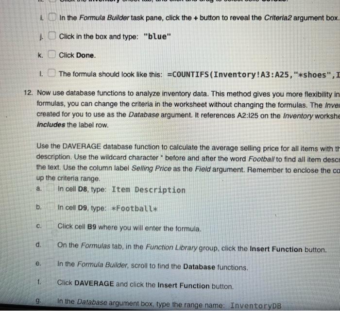
1. Open the start file EX2019-SkillReview-6-2. The file will be renamed automatically to include your name file name if directed to do so by your instructor, and save it. 2. If the workbook opens in Protected View, click the Enable Editing button in the Message Bar at the top can modify the workbook. NOTE: If group titles are not visible on your Ribbon in Excel for Mac, click the Excel menu and select Preferenc Preferences dialog box. Click the View button and check the Group Titles check box under in Ribbon, Show. C Preferences dialog box. 3. Start with the Inventory worksheet. Use the LEFT function to extract the category ID from the inventory numbe a. Click in cell F3. b. Type: =LEFT ( c. Click cell B3. d. Type: , 2) e. The formula should look like this: =LEFT (B3,2) t. Copy the formula to cells F4:F25. 4. Switch to the Analysis worksheet. Use the SUMPRODUCT function to calculate the total value of the inventory. the Selling Price column and the corresponding values in the Stock column as the Array arguments. a. Click cell B2. b. Type: =SUMPRODUCT ( c. Click the Inventory sheet tab, and then click and drag to select cells H3:H25. d. Type , and then click and drag to select cells 13:125. e. Type ) and press f. The formula should look like this: =SUMPRODUCT (Inventory ! H3: H25, Inventory! I3: I25) 5. Enter a formula to calculate the average selling price. a. Click cell D2. b. Type: =AVERAGE ( c. Click the Inventory sheet tab, and then click and drag to select cells H3:H25. d. Press The formula should look like this: =AVERAGE (Inventory ! H3:H25) 6. Enter a formula to find the middle selling price. a. Click cell E2. b. Type: =MEDIAN ( c. Click the Inventory sheet tab, and then click and drag to select cells H3:H25. d. Press The formula should look like this: =MEDIAN (Inventory ! H3: H25) 7. Enter a formula to find the most common selling price. a. Click cell F2. b. Type: =MODE. SNGL ( c. Click the Inventory sheet tab, and then click and drag to select cells H3:H25. d. Press The formula should look like this: d. Press The formula should look like this: =MODE. SNGL (Inventory IH3:H25) 8. What if there are multiple selling prices that are the most common? Enter an array formula common selling prices. a. Select cells G2:G5. b. Type: =MODE.MULT( c. Click the Inventory sheet tab, and then click and drag to select cells H3:H25. d. Press Control + Shitt + Enter. The formula should look like this: {= MODE.MULT (Inventory ! H3: H25) \} 9. Use the SUMIFS function to calculate the total number of blue shoes in inventory. Use the val Sum_range argument. Use the values in the Item Description column as the Criteria_ranget a to find all items that end in the word shoes. Use the values in the Color column as the Criteria criteria blue. a. Click cell B3. b. On the Formulas tab, in the Function Library group, click the Math \& Trig button and seli c. In the Formula Builder task pane, verify that the cursor is in the Sum_range argument bo and click and drag to select cells 13:125. d. In the Formula Builder task pane, click the + button to reveal the Criteria ranget argumer e. Click in the Criteria range 1 box and click the Inventory sheet tab, and click and drag to s f. In the Formula Builder task pane, click the + button to reveal the Criteriat argument box. j. In the Formula Builder task pane, Click the + button to reveal to the Criteria2 argumen k. Click in the Criteria2 box and type: "blue" I. Click Done. m. The formula should look like this: =SUMIFS (Inventory! I3: I25, Inventory ! A3:A25, "*shoes", Inventoi 10. Use the AVERAGEIFS function to find the average selling price of blue shoes in inventory. Us column as the Average_range argument. Use the values in the Item Description column as the the criteria "shoes to find all items that end in the word shoes. Use the values in the Color colt and use the criteria blue. a. Click cell B4. b. On the Formulas tab, in the Function Library group, click the More Functions button, p AVERAGEIFS. c. In the Formula Builder task pane, verify that the cursor is in the Average_range argume tab, and click and drag to select cells H3:H25. d. In the Formula Builder task pane, click the + button to reveal the Criteria_range1 argum e. Click in the Criteria_range1 box and click the Inventory sheet tab. Click and drag to sele f. In the Formula Builder task pane, click the + button to reveal the Criteriat argument box. g. Click in the Criteria 1 box and type "*shoes" to find any text string that ends with the h. Press the + button to reveal the Criteria range2 argument box and click in the box. i. In the Formula Builder task pane, click the + button to reveal the Criteria2 argument box. j. Click in the box and type: "blue" k. Click Done. 1. The formula should look like this: =COUNTIFS (Inventory ! A3:A25, "*shoes", I 12. Now use database functions to analyze inventory data. This method gives you more flexibility in formulas, you can change the criteria in the worksheet without changing the formulas. The Invel created for you to use as the Database argument. It references A2:I25 on the inventory workshe includes the label row. Use the DAVERAGE database function to calculate the average selling price for all items with th description. Use the wildcard character " before and after the word Football to find all item desci the text. Use the column label Selling Price as the Field argument. Remember to enclose the co up the criteria range. a. In cell D8, type: Item Description b. In cell D9, type: *FootbaLl* c. Click cell B9 where you will enter the formula. d. On the Formulas tab, in the Function Library group, click the Insert Function button. e. In the Formula Builder, scroll to tind the Database functions. f. Click DAVERAGE and click the Insert Function button