

Question: Stack the data in the Stacked worksheet. 1 : Preparation Step 1 : The CRSP Data worksheet has data for the largest companies in nineteen
Stack the data in the Stacked worksheet.
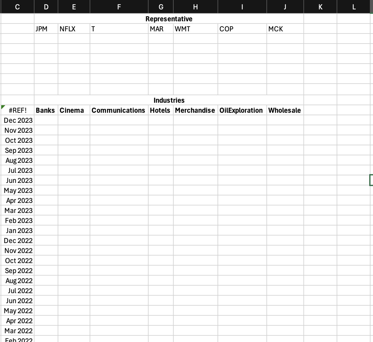
: Preparation
Step : The CRSP Data worksheet has data for the largest
companies in nineteen industries for every month for ten years.
Step : Type your first name and Net ID into Cells A:B on the
Stacked worksheet.
Step : Replace the inputs in Cells D:J on the Stacked
worksheet with the names of your industries, keep the order.
Step : Create a formula in Cell D on the Stacked worksheet that
finds the representative ticker for the industries in D
Step : CopyPaste this formula such that the representative
tickers appear for Cells E:J
Step : Change the formatting for the months, Cells C:C to
match that on the CRSP Data worksheet.
: Complete Table
Step : Use the Data Table tool to fill in the table, Cells D:J
with the returns for the industry in the months given.
Step : Make the formatting display for the returns
B Paste the data in the Betas worksheet
Step : Use the Data Validation tool to create a dropdown menu
for Cell C on the Betas worksheet to select from, and only from, one
of the months in
Step : Change the formatting for Cell C to match that on the
CRSP Data worksheet.
Step : Create a formula in Cell D that will get the beta for the
Industry in D for the five years immediately preceding the month
selected in Cell C To receive full credit, this formula needs to adjust
automatically for any of the twelve possible months in Cell C
Step : CopyPaste this formula from Cell D to E:J
Step : The formatting for the betas needs to be as they are
normally displayed.
B Performance Evaluation
Step : Create a formula for Cell D that computes the Alpha for
the Industry in Cell D for the five years immediately preceding the
month selected in Cell C To receive full credit, this formula needs to
adjust automatically for any of the twelve possible months in Cell C
Step : Create a formula for Cell D that computes the Treynor
Ratio for the Industry in Cell D for the five years immediately
preceding the month selected in Cell C To receive full credit, this
formula needs to adjust automatically for any of the twelve possible
months in Cell C
Step : CopyPaste these formulas from Cells D:D to E:J
Step : The formatting for the two performance evaluation
measures must be as they are normally displayed.
Step by Step Solution
There are 3 Steps involved in it
1 Expert Approved Answer
Step: 1 Unlock

Question Has Been Solved by an Expert!
Get step-by-step solutions from verified subject matter experts
Step: 2 Unlock
Step: 3 Unlock