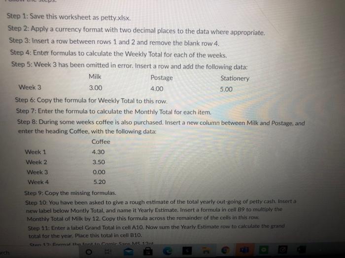
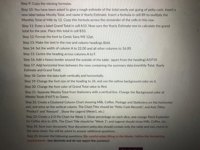
Step 1: Save this worksheet as petty.xlsx Step 2: Apply a currency format with two decimal places to the data where appropriate. Step 3: Insert a row between rows 1 and 2 and remove the blank row 4. Step 4: Enter formulas to calculate the Weekly Total for each of the weeks. Step 5: Week 3 has been omitted in error. Insert a row and add the following data: Milk Postage Stationery Week 3 3.00 4.00 5.00 Step 6: Copy the formula for Weekly Total to this row. Step 7: Enter the formula to calculate the Monthly Total for each item. Step 8: During some weeks coffee is also purchased. Insert a new column between Milk and Postage, and enter the heading Coffee, with the following data: Coffee 4.30 Week 1 Week 2 Week 3 Week 4 3.50 0.00 5.20 Step 9: Copy the missing formulas. Step 10: You have been asked to give a rough estimate of the total yearly out-going of petty cash. Insert a new label below Montly Total, and name it Yearly Estimate. Insert a formula in cell B9 to multiply the Monthly Total of Milk by 12. Copy this formula across the remainder of the cells in this row. Step 11: Enter a label Grand Total in cell A10. Now sum the Yearly Estimate row to calculate the grand total for the year. Place this total in cell B10. 12. Fremst the tanto Comic Sans MS 12 O ch Step 9: Copy the missing formulas. Step 10: You have been asked to give a rough estimate of the total yearly out-going of petty cash. Insert a new label below Montly Total, and name it Yearly Estimate. Insert a formula in cell B9 to multiply the Monthly Total of Milk by 12. Copy this formula across the remainder of the cells in this row. Step 11: Enter a label Grand Total in cell A10. Now sum the Yearly Estimate row to calculate the grand total for the year. Place this total in cell B10. Step 12: Format the font to Comic Sans MS 12pt. Step 13: Make the text in the row and column headings Bold, Step 14: Set the width of column A to 22.00 and all other columns to 16.00. Step 15: Centre the heading across columns A to F. Step 16: Add a heavy border around the outside of the table (apart from the heading) A3:F10 Step 17: Add horizontal lines between the rows containing the summary data (monthly Total. Yearly Estimate and Grand Total). Step 18: Center the data both vertically and horizontally. Step 19: Change the font size of the heading to 24 and use the yellow background color on it. Step 20: Change the font color of Grand Total value to Red. Step 21: Separate Weekly Total from Stationery with a vertical fine. Change the Background color of Weekly Totals (F4:F7) to Green. Step 22: Create a Clustered Column Chart showing Milk Coffee, Postage and Stationery on the horizontal axis, and price on the vertical column. The Chart Title should be "Petty Cash Records", and Axis Titles: "Product" and "Amount". Show the Legend (Week1. etc.) Step 23: Create a 2-D Pie Chart for Week 1. Show percentage on each slice, and change Point Explosion for Coffee slice to 20%. The Chart Title should be "Week 15 and Legend should show Milk, Coffee, etc. Step 24: Save your document. Your document petty.xlsx should contain only the table and two charts in the same sheet. You will be asked to answer additional questions Step 25: Answer the following questions: (Be careful when filling in the blanks follow the formatting requirements-two decimals and do not report the currency Step 1: Save this worksheet as petty.xlsx Step 2: Apply a currency format with two decimal places to the data where appropriate. Step 3: Insert a row between rows 1 and 2 and remove the blank row 4. Step 4: Enter formulas to calculate the Weekly Total for each of the weeks. Step 5: Week 3 has been omitted in error. Insert a row and add the following data: Milk Postage Stationery Week 3 3.00 4.00 5.00 Step 6: Copy the formula for Weekly Total to this row. Step 7: Enter the formula to calculate the Monthly Total for each item. Step 8: During some weeks coffee is also purchased. Insert a new column between Milk and Postage, and enter the heading Coffee, with the following data: Coffee 4.30 Week 1 Week 2 Week 3 Week 4 3.50 0.00 5.20 Step 9: Copy the missing formulas. Step 10: You have been asked to give a rough estimate of the total yearly out-going of petty cash. Insert a new label below Montly Total, and name it Yearly Estimate. Insert a formula in cell B9 to multiply the Monthly Total of Milk by 12. Copy this formula across the remainder of the cells in this row. Step 11: Enter a label Grand Total in cell A10. Now sum the Yearly Estimate row to calculate the grand total for the year. Place this total in cell B10. 12. Fremst the tanto Comic Sans MS 12 O ch Step 9: Copy the missing formulas. Step 10: You have been asked to give a rough estimate of the total yearly out-going of petty cash. Insert a new label below Montly Total, and name it Yearly Estimate. Insert a formula in cell B9 to multiply the Monthly Total of Milk by 12. Copy this formula across the remainder of the cells in this row. Step 11: Enter a label Grand Total in cell A10. Now sum the Yearly Estimate row to calculate the grand total for the year. Place this total in cell B10. Step 12: Format the font to Comic Sans MS 12pt. Step 13: Make the text in the row and column headings Bold, Step 14: Set the width of column A to 22.00 and all other columns to 16.00. Step 15: Centre the heading across columns A to F. Step 16: Add a heavy border around the outside of the table (apart from the heading) A3:F10 Step 17: Add horizontal lines between the rows containing the summary data (monthly Total. Yearly Estimate and Grand Total). Step 18: Center the data both vertically and horizontally. Step 19: Change the font size of the heading to 24 and use the yellow background color on it. Step 20: Change the font color of Grand Total value to Red. Step 21: Separate Weekly Total from Stationery with a vertical fine. Change the Background color of Weekly Totals (F4:F7) to Green. Step 22: Create a Clustered Column Chart showing Milk Coffee, Postage and Stationery on the horizontal axis, and price on the vertical column. The Chart Title should be "Petty Cash Records", and Axis Titles: "Product" and "Amount". Show the Legend (Week1. etc.) Step 23: Create a 2-D Pie Chart for Week 1. Show percentage on each slice, and change Point Explosion for Coffee slice to 20%. The Chart Title should be "Week 15 and Legend should show Milk, Coffee, etc. Step 24: Save your document. Your document petty.xlsx should contain only the table and two charts in the same sheet. You will be asked to answer additional questions Step 25: Answer the following questions: (Be careful when filling in the blanks follow the formatting requirements-two decimals and do not report the currency