stuck at step 4, please answer step 4 and rest

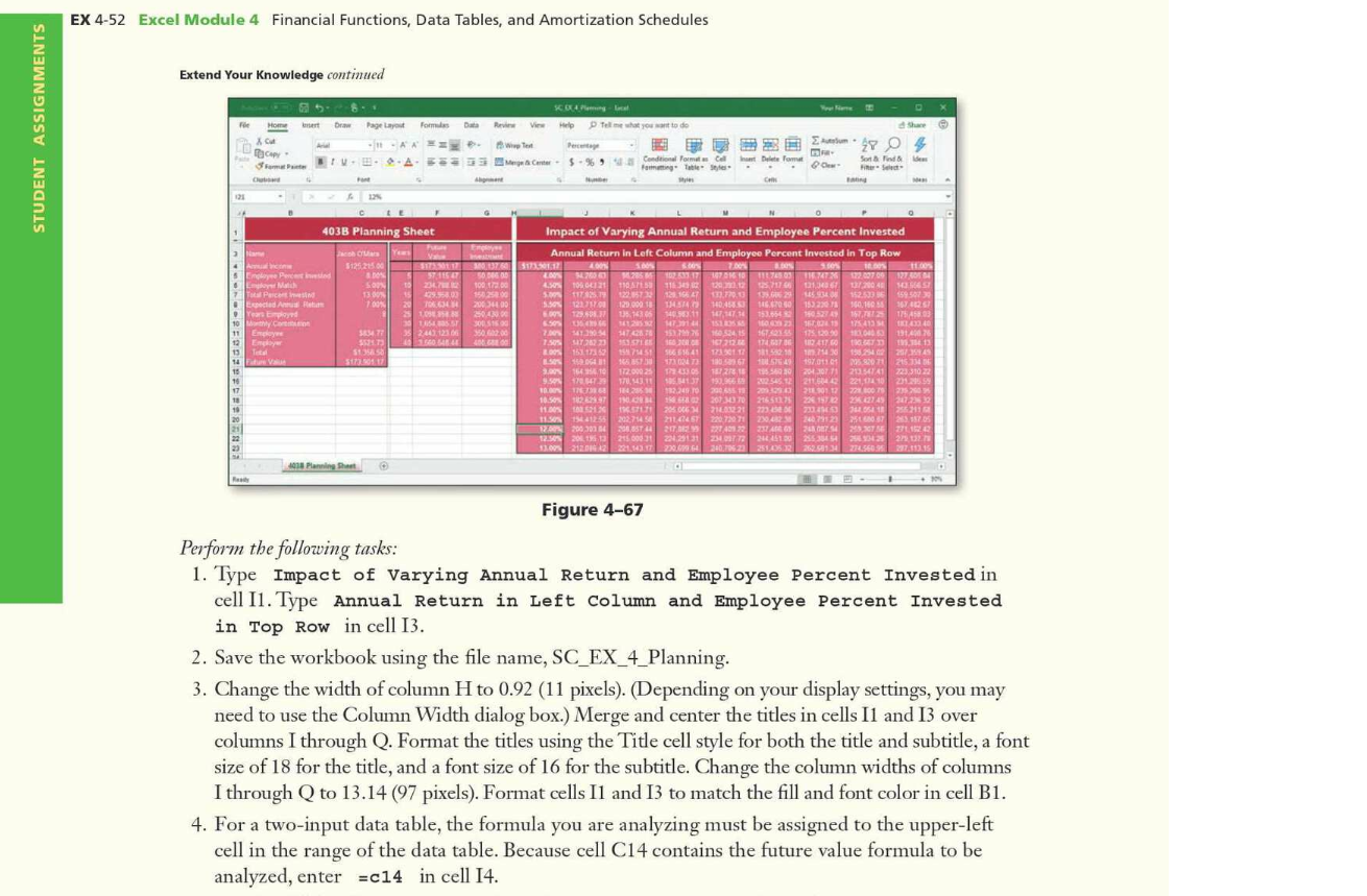
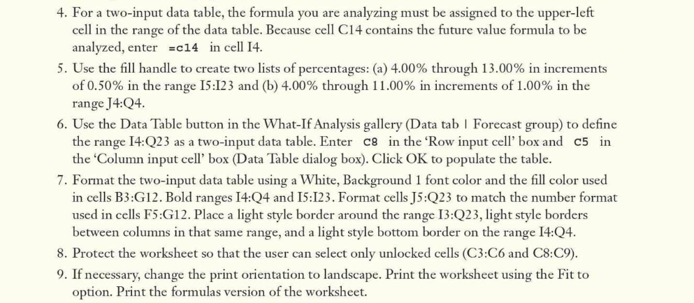
EX 4-52 Excel Module 4 Financial Functions, Data Tables, and Amortization Schedules Extend Your Knowledge continued 5 ent Home STUDENT ASSIGNMENTS Draw X Copy Komuna Page Layout Fomus Data Rev Vie Help Delme what you want to do - 11-AA Who Peca 2.452 53 Center 5.9 $ - % 9 Conditional Format Home Tole A BV Share m 0 het Delete com Sort & Tinde 121 403B Planning Sheet Em Calle ya 5125215313 312 SON 13 700 10 151 25. KOU 10 100 1520 200340 3504300 BOSS 35 2449.1234 2 S Employee Peed . Low Maio 7 Telecentes Espected Ant Years Employed 10.com 11E Engiya 19 Emy 13 Teto 10 18 16 17 12 10 20 21 3477 $575. 51 Impact of varying Annual Return and Employee Percent Invested Annual Return in Left Column and Employee Percent Invested in Top Row 20 5. 7.be . 16.00 11.00 2003 2002 102 WRITTEN 1 45 TO 11 AT 1163 2166 2006 2004 HOS 1178353 123 1664 13.770.0 25 145.31 152.53 159592 12231701 129.000 11454 140.45 153 2018 160.10 904025 800 123.583.3.16386 149.5311147 1474 153.0543 15. 1754 6.5 1125 11 16.04.13 D40 2.447.78 1517160534, 5 16721 10 1514 1.50 222 1537 16.01072 1747 12 411 6 TO GET 11 200 15173 17451 SE641 1311 13150 1011 158251 2012249 12064 165857 1967 1764 17.011 M82071215334 2.0 164410 172.00025 12.30 1072 600 20120711 2014 9.178.147.29 170.14311 0541.37 190,966 2545.12 211.60 221,11210 2012 10 11 12 112.2402006951 2950 2011 2010 257 IT IN . 156 207 3070 216.50 23245 247.2222 11.00 15.12 IKS 2006 221 222 2201 2110 11. 1964125 202.754 54 201047 220 7221 2704224079523 LES 120 200 300 GAST 44 27, 221401 22 23 2 GETS KTM 12. 2018 21500231 2012013122410 2353454 201 13.00 21.142.17 29.04.20,7062251.035 R 26258134 274.560.93 20111315 . 20 4018 Planning Short Figure 4-67 Perform the following tasks: 1. Type Impact of varying Annual Return and Employee Percent Invested in cell I1. Type Annual Return in Left Column and Employee Percent Invested in Top Row in cell 13. 2. Save the workbook using the file name, SC_EX_4_Planning. 3. Change the width of column H to 0.92 (11 pixels). (Depending on your display settings, you may need to use the Column Width dialog box.) Merge and center the titles in cells I1 and 13 over columns I through Q. Format the titles using the Title cell style for both the title and subtitle, a font size of 18 for the title, and a font size of 16 for the subtitle. Change the column widths of columns I through Q to 13.14 (97 pixels). Format cells II and 13 to match the fill and font color in cell B1. 4. For a two-input data table, the formula you are analyzing must be assigned to the upper-left cell in the range of the data table. Because cell C14 contains the future value formula to be analyzed, enter =c14 in cell 14. 4. For a two-input data table, the formula you are analyzing must be assigned to the upper-left cell in the range of the data table. Because cell C14 contains the future value formula to be analyzed, enter EC14 in cell 14. 5. Use the fill handle to create two lists of percentages: (a) 4.00% through 13.00% in increments of 0.50% in the range 15:12 3 and (b) 4.00% through 11.00% in increments of 1.00% in the range J4:Q4. 6. Use the Data Table button in the What-If Analysis gallery (Data tab | Forecast group) to define the range 14:Q23 as a two-input data table. Enter C8 in the Row input cell box and c5 in the 'Column input cell box (Data Table dialog box). Click OK to populate the table. 7. Format the two-input data table using a White, Background 1 font color and the fill color used in cells B3:G12. Bold ranges 14:Q4 and 15:123. Format cells J5:Q23 to match the number format used in cells F5:G12. Place a light style border around the range 13:Q23, light style borders between columns in that same range, and a light style bottom border on the range 14:Q4. 8. Protect the worksheet so that the user can select only unlocked cells (C3:C6 and C8:C9). 9. If necessary, change the print orientation to landscape. Print the worksheet using the Fit to option. Print the formulas version of the worksheet. EX 4-52 Excel Module 4 Financial Functions, Data Tables, and Amortization Schedules Extend Your Knowledge continued 5 ent Home STUDENT ASSIGNMENTS Draw X Copy Komuna Page Layout Fomus Data Rev Vie Help Delme what you want to do - 11-AA Who Peca 2.452 53 Center 5.9 $ - % 9 Conditional Format Home Tole A BV Share m 0 het Delete com Sort & Tinde 121 403B Planning Sheet Em Calle ya 5125215313 312 SON 13 700 10 151 25. KOU 10 100 1520 200340 3504300 BOSS 35 2449.1234 2 S Employee Peed . Low Maio 7 Telecentes Espected Ant Years Employed 10.com 11E Engiya 19 Emy 13 Teto 10 18 16 17 12 10 20 21 3477 $575. 51 Impact of varying Annual Return and Employee Percent Invested Annual Return in Left Column and Employee Percent Invested in Top Row 20 5. 7.be . 16.00 11.00 2003 2002 102 WRITTEN 1 45 TO 11 AT 1163 2166 2006 2004 HOS 1178353 123 1664 13.770.0 25 145.31 152.53 159592 12231701 129.000 11454 140.45 153 2018 160.10 904025 800 123.583.3.16386 149.5311147 1474 153.0543 15. 1754 6.5 1125 11 16.04.13 D40 2.447.78 1517160534, 5 16721 10 1514 1.50 222 1537 16.01072 1747 12 411 6 TO GET 11 200 15173 17451 SE641 1311 13150 1011 158251 2012249 12064 165857 1967 1764 17.011 M82071215334 2.0 164410 172.00025 12.30 1072 600 20120711 2014 9.178.147.29 170.14311 0541.37 190,966 2545.12 211.60 221,11210 2012 10 11 12 112.2402006951 2950 2011 2010 257 IT IN . 156 207 3070 216.50 23245 247.2222 11.00 15.12 IKS 2006 221 222 2201 2110 11. 1964125 202.754 54 201047 220 7221 2704224079523 LES 120 200 300 GAST 44 27, 221401 22 23 2 GETS KTM 12. 2018 21500231 2012013122410 2353454 201 13.00 21.142.17 29.04.20,7062251.035 R 26258134 274.560.93 20111315 . 20 4018 Planning Short Figure 4-67 Perform the following tasks: 1. Type Impact of varying Annual Return and Employee Percent Invested in cell I1. Type Annual Return in Left Column and Employee Percent Invested in Top Row in cell 13. 2. Save the workbook using the file name, SC_EX_4_Planning. 3. Change the width of column H to 0.92 (11 pixels). (Depending on your display settings, you may need to use the Column Width dialog box.) Merge and center the titles in cells I1 and 13 over columns I through Q. Format the titles using the Title cell style for both the title and subtitle, a font size of 18 for the title, and a font size of 16 for the subtitle. Change the column widths of columns I through Q to 13.14 (97 pixels). Format cells II and 13 to match the fill and font color in cell B1. 4. For a two-input data table, the formula you are analyzing must be assigned to the upper-left cell in the range of the data table. Because cell C14 contains the future value formula to be analyzed, enter =c14 in cell 14. 4. For a two-input data table, the formula you are analyzing must be assigned to the upper-left cell in the range of the data table. Because cell C14 contains the future value formula to be analyzed, enter EC14 in cell 14. 5. Use the fill handle to create two lists of percentages: (a) 4.00% through 13.00% in increments of 0.50% in the range 15:12 3 and (b) 4.00% through 11.00% in increments of 1.00% in the range J4:Q4. 6. Use the Data Table button in the What-If Analysis gallery (Data tab | Forecast group) to define the range 14:Q23 as a two-input data table. Enter C8 in the Row input cell box and c5 in the 'Column input cell box (Data Table dialog box). Click OK to populate the table. 7. Format the two-input data table using a White, Background 1 font color and the fill color used in cells B3:G12. Bold ranges 14:Q4 and 15:123. Format cells J5:Q23 to match the number format used in cells F5:G12. Place a light style border around the range 13:Q23, light style borders between columns in that same range, and a light style bottom border on the range 14:Q4. 8. Protect the worksheet so that the user can select only unlocked cells (C3:C6 and C8:C9). 9. If necessary, change the print orientation to landscape. Print the worksheet using the Fit to option. Print the formulas version of the worksheet