$\backslash$table$[[,$Year $1,$Year $2,$Year $3,$Year $4,$Year $5,$Year $6],[$Beginning book value,$$100,000,$$$93,300,$$$91,600,$$$89,900,\backslash$table$[[$$$85,700$

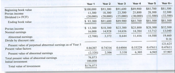
To show that Ford would get exactly the same result using an abnormal earnings approach, we illustrate that approach in Exhibit $7\mathrm{.}7.$ We take care to ensure that the assumptions we make in this exhibit, which are formulated in terms of earnings and book values, are consistent with the cash flows we obtained in Exhibit $7\mathrm{.}6.$ First we determine the investment's book value of equity each year. For each year, we can take beginning book value, add pretax income, and subtract dividends. We have already determined pretax income for each period. Dividends are set to the amount of free cash flow generated during the year, because this represents the amount of cash that could be taken out of the business without affecting its ability to generate the future cash flows in the forecast. So$,$ for example, in Year $1,$ equity book value declines by $$6,700$ because the dividend exceeds pre$-$tax income by that amount. The resulting book value of $$93,300$ becomes the beginning book value for the next year, and the process is repeated.

We multiply the beginning book value in each period by $16\%($the cost of capital$)$ to determine the level of normal earnings for the year. When we subtract that amount from actual pre$-$tax income, we have abnormal earnings. Note that abnormal carnings also settle at a constant level$-$$$19\mathrm{.}460-$allowing us once again to compute the present value of an infinite series. The present

value of the abnormal earnings is $$76,873,$ resulting in an investment value of $$176,873.$ Because we used assumptions that are equivalent in the approaches, the results were identical.

Another word about valuations is appropriate here. Valuation professionals often treat cash flows as if they occur at midyear, in order to approximate more closely cash flows that occur throughout the year. This treatment is accomplished by discounting cash flows for $0\mathrm{.}5$ year, $1\mathrm{.}5$ years. $....$ or by use of a "midyear adjustment" to the present value as it is computed in Exhibit $7\mathrm{.}6.$ The midyear adjustment is to multiply the present value in the exhibit by the square root of one plus the discount rate. In our example, the adjustment results in a present value of $$176,873*\sqrt[\phantom{2}]{1,16}=$$$190,498.$