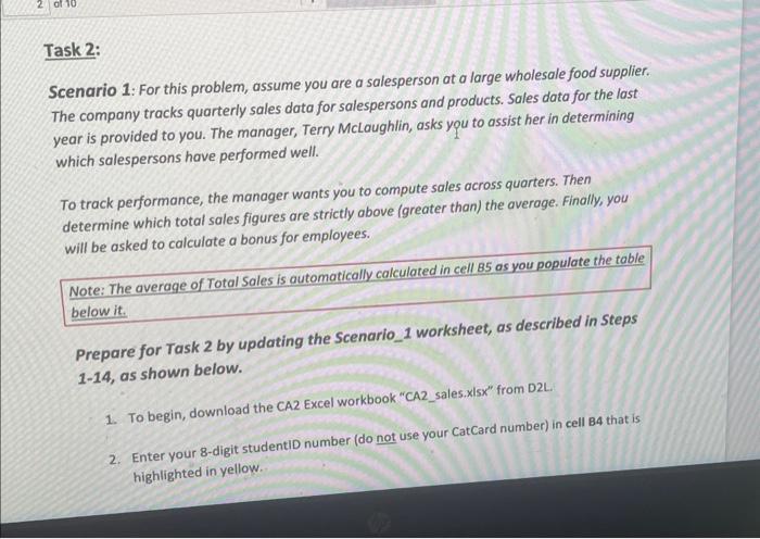
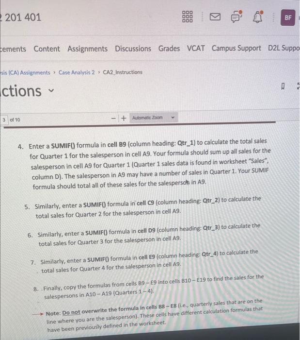
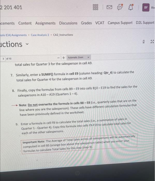
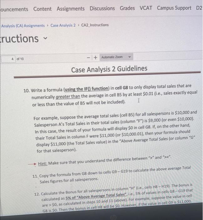
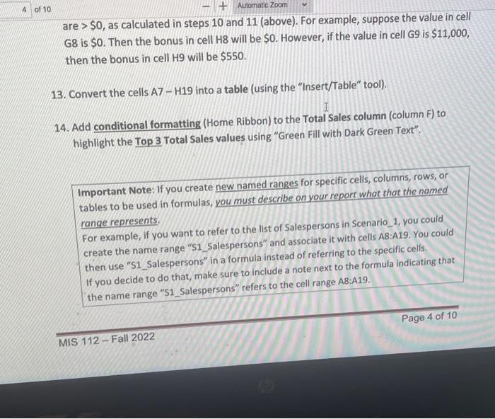
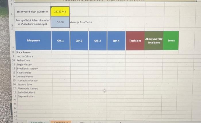
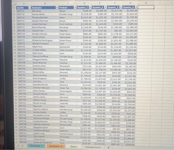
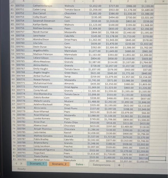
Task 2: Scenario 1: For this problem, assume you are a salesperson at a large wholesale food supplier. The company tracks quarterly sales data for salespersons and products. Sales data for the last year is provided to you. The manager, Terry Mclaughlin, asks you to assist her in determining which salespersons have performed well. To track performance, the manager wants you to compute sales across quarters. Then determine which total sales figures are strictly above (greater than) the average. Finally, you will be asked to calculate a bonus for employees. Note: The average of Total Sales is automatically calculated in cell 85 as you populate the table below it. Prepare for Task 2 by updating the Scenario_ 1 worksheet, as described in Steps 1-14, as shown below. 1. To begin, download the CA2 Excel workbook "CA2_sales.xlsx" from D2L. 2. Enter your 8-digit studentiD number (do not use your CatCard number) in cell B4 that is highlighted in yellow. 4. Enter a SUMIF() formula in cell B9 (column heading: Qtr_1) to calculate the total sales for Quarter 1 for the salesperson in cell A9. Your formula should sum up all sales for the salesperson in cell A9 for Quarter 1 (Quarter 1 sales data is found in worksheet "Sales", column D). The salesperson in A9 may have a number of sales in Quarter 1. Your SUMIF formula should total all of these sales for the salespersot in A9. 5. Similarly, enter a SUMIF() formula in cell C9 (column heading: Qtr_2) to calculate the total sales for Quarter 2 for the salesperson in cell A9. 6. Similarly, enter a SUMIF() formula in cell D9 (column heading: Qtr_3) to calculate the total sales for Quarter 3 for the salesperson in cell A.9. 7. Similarly, enter a SUMIF() formula in cell E9 (column heading: Qtr_4) to calculate the total sales for Quarter 4 for the salesperson in cell A9. 8. Finally, copy the formulas from cells B9 - E9 into cells B10-E19 to find the sales for the salespersons in A10-A19 (Quarters 1 - 4). Note: Do not overwrite the formula in cells B8 - E8 (i.e., quarterly sales that are on the line where you are the salesperson). These cells have different calculation formulas that have been previously defined in the worksheet. total sales for Quarter 3 for the salesperson in cell A9. 7. Similarly, enter a SUMIF) formula in cell E9 (column heading: Qtr_4) to calculate the total sales for Quarter 4 for the salesperson in cell A9. 8. Finally, copy the formulas from cells B9 - E9 into cells B10 - E19 to find the sales for the salespersons in A10-A19 (Quarters 1 - 4). Note: Do not overwrite the formula in cells B8 - E8 (i.e., quarterly sales that are on the line where you are the salesperson). These cells have different calculation formulas that have been previously defined in the worksheet. 9. Enter a formula in cell F8 to calculate the total sales (i.e., a summation of sales in Quarter 1- Quarter 4). Copy this formula into cells F9. F19 to calculate total sales for each of the other salespersons. Important Note: The Average of Total Sales across all salespersons will be automatically, computed in cell B5 (orange box above the salesperson table) when you enter your formulas to calculate Total Sales for this step (step 9). 10. Write a formula (using the IF() function) in cell G8 to only display total sales that are numerically greater than the average in cell B5 by at least $0.01 (i.e., sales exactly equal or less than the value of B5 will not be included). For example, suppose the average total sales (cell B5) for all salespersons is $10,000 and Salesperson A's Total Sales in their total sales (column " F ") is $9,000 (or even $10,000 ). In this case, the result of your formula will display $0 in cell G8. If, on the other hand, their Total Sales in column F were $11,000 (or $10,000.01 ), then your formula should display $11,000 (the Total Sales value) in the "Above Average Total Sales (or column " G " for that salesperson). Hint; Make sure that you understand the difference between " > " and " >=". 11. Copy the formula from G8 down to cells G9 - G19 to calculate the above average Total Sales figures for all salespersons. 12. Calculate the Bonus for all salespersons in column "H" (i.e., cells HBH19). The bonus is calculated as 5% of "Above Average Total Sales", i.e., 5% of values in cells G8 - G19 that are >$0, as calculated in steps 10 and 11 (above). For example, suppose the value in cell are >$0, as calculated in steps 10 and 11 (above). For example, suppose the value in cell G8 is $0. Then the bonus in cell H8 will be $0. However, if the value in cell G9 is $11,000, then the bonus in cell Hg will be $550. 13. Convert the cells A7 - H19 into a table (using the "Insert/Table" tool). 14. Add conditional formatting (Home Ribbon) to the Total Sales column (column F) to highlight the Top 3 Total Sales values using "Green Fill with Dark Green Text". 3 \begin{tabular}{|l|l|l|l|} \hline 4 & Enteryour 8-digit studentio & 23793748 & \\ \hline & Average Total Soles calculated & 50.00 & \\ \hline 5 & in shaded boxon the right & & \\ \hline 6 & & \\ \hline \end{tabular} Task 2: Scenario 1: For this problem, assume you are a salesperson at a large wholesale food supplier. The company tracks quarterly sales data for salespersons and products. Sales data for the last year is provided to you. The manager, Terry Mclaughlin, asks you to assist her in determining which salespersons have performed well. To track performance, the manager wants you to compute sales across quarters. Then determine which total sales figures are strictly above (greater than) the average. Finally, you will be asked to calculate a bonus for employees. Note: The average of Total Sales is automatically calculated in cell 85 as you populate the table below it. Prepare for Task 2 by updating the Scenario_ 1 worksheet, as described in Steps 1-14, as shown below. 1. To begin, download the CA2 Excel workbook "CA2_sales.xlsx" from D2L. 2. Enter your 8-digit studentiD number (do not use your CatCard number) in cell B4 that is highlighted in yellow. 4. Enter a SUMIF() formula in cell B9 (column heading: Qtr_1) to calculate the total sales for Quarter 1 for the salesperson in cell A9. Your formula should sum up all sales for the salesperson in cell A9 for Quarter 1 (Quarter 1 sales data is found in worksheet "Sales", column D). The salesperson in A9 may have a number of sales in Quarter 1. Your SUMIF formula should total all of these sales for the salespersot in A9. 5. Similarly, enter a SUMIF() formula in cell C9 (column heading: Qtr_2) to calculate the total sales for Quarter 2 for the salesperson in cell A9. 6. Similarly, enter a SUMIF() formula in cell D9 (column heading: Qtr_3) to calculate the total sales for Quarter 3 for the salesperson in cell A.9. 7. Similarly, enter a SUMIF() formula in cell E9 (column heading: Qtr_4) to calculate the total sales for Quarter 4 for the salesperson in cell A9. 8. Finally, copy the formulas from cells B9 - E9 into cells B10-E19 to find the sales for the salespersons in A10-A19 (Quarters 1 - 4). Note: Do not overwrite the formula in cells B8 - E8 (i.e., quarterly sales that are on the line where you are the salesperson). These cells have different calculation formulas that have been previously defined in the worksheet. total sales for Quarter 3 for the salesperson in cell A9. 7. Similarly, enter a SUMIF) formula in cell E9 (column heading: Qtr_4) to calculate the total sales for Quarter 4 for the salesperson in cell A9. 8. Finally, copy the formulas from cells B9 - E9 into cells B10 - E19 to find the sales for the salespersons in A10-A19 (Quarters 1 - 4). Note: Do not overwrite the formula in cells B8 - E8 (i.e., quarterly sales that are on the line where you are the salesperson). These cells have different calculation formulas that have been previously defined in the worksheet. 9. Enter a formula in cell F8 to calculate the total sales (i.e., a summation of sales in Quarter 1- Quarter 4). Copy this formula into cells F9. F19 to calculate total sales for each of the other salespersons. Important Note: The Average of Total Sales across all salespersons will be automatically, computed in cell B5 (orange box above the salesperson table) when you enter your formulas to calculate Total Sales for this step (step 9). 10. Write a formula (using the IF() function) in cell G8 to only display total sales that are numerically greater than the average in cell B5 by at least $0.01 (i.e., sales exactly equal or less than the value of B5 will not be included). For example, suppose the average total sales (cell B5) for all salespersons is $10,000 and Salesperson A's Total Sales in their total sales (column " F ") is $9,000 (or even $10,000 ). In this case, the result of your formula will display $0 in cell G8. If, on the other hand, their Total Sales in column F were $11,000 (or $10,000.01 ), then your formula should display $11,000 (the Total Sales value) in the "Above Average Total Sales (or column " G " for that salesperson). Hint; Make sure that you understand the difference between " > " and " >=". 11. Copy the formula from G8 down to cells G9 - G19 to calculate the above average Total Sales figures for all salespersons. 12. Calculate the Bonus for all salespersons in column "H" (i.e., cells HBH19). The bonus is calculated as 5% of "Above Average Total Sales", i.e., 5% of values in cells G8 - G19 that are >$0, as calculated in steps 10 and 11 (above). For example, suppose the value in cell are >$0, as calculated in steps 10 and 11 (above). For example, suppose the value in cell G8 is $0. Then the bonus in cell H8 will be $0. However, if the value in cell G9 is $11,000, then the bonus in cell Hg will be $550. 13. Convert the cells A7 - H19 into a table (using the "Insert/Table" tool). 14. Add conditional formatting (Home Ribbon) to the Total Sales column (column F) to highlight the Top 3 Total Sales values using "Green Fill with Dark Green Text". 3 \begin{tabular}{|l|l|l|l|} \hline 4 & Enteryour 8-digit studentio & 23793748 & \\ \hline & Average Total Soles calculated & 50.00 & \\ \hline 5 & in shaded boxon the right & & \\ \hline 6 & & \\ \hline \end{tabular}