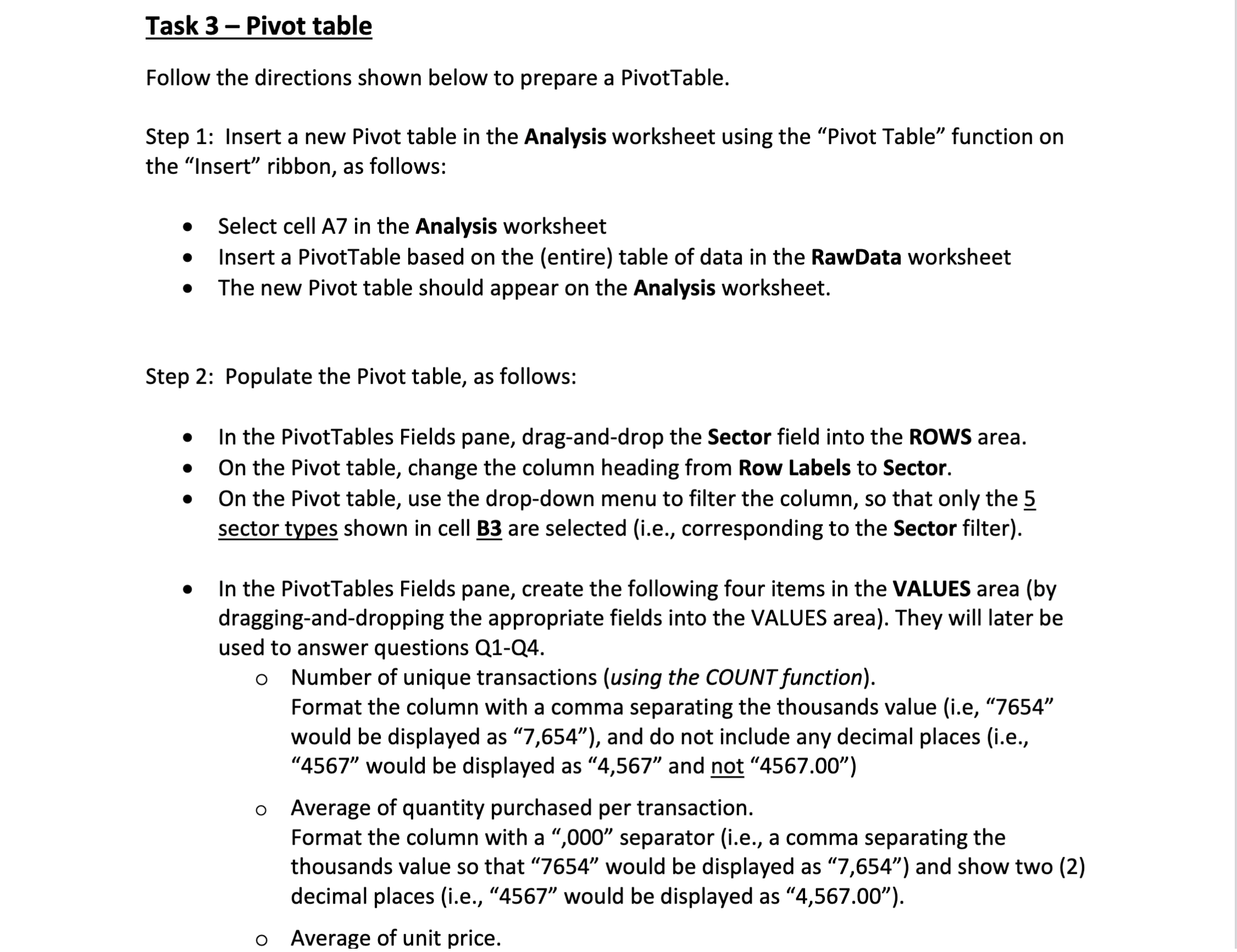
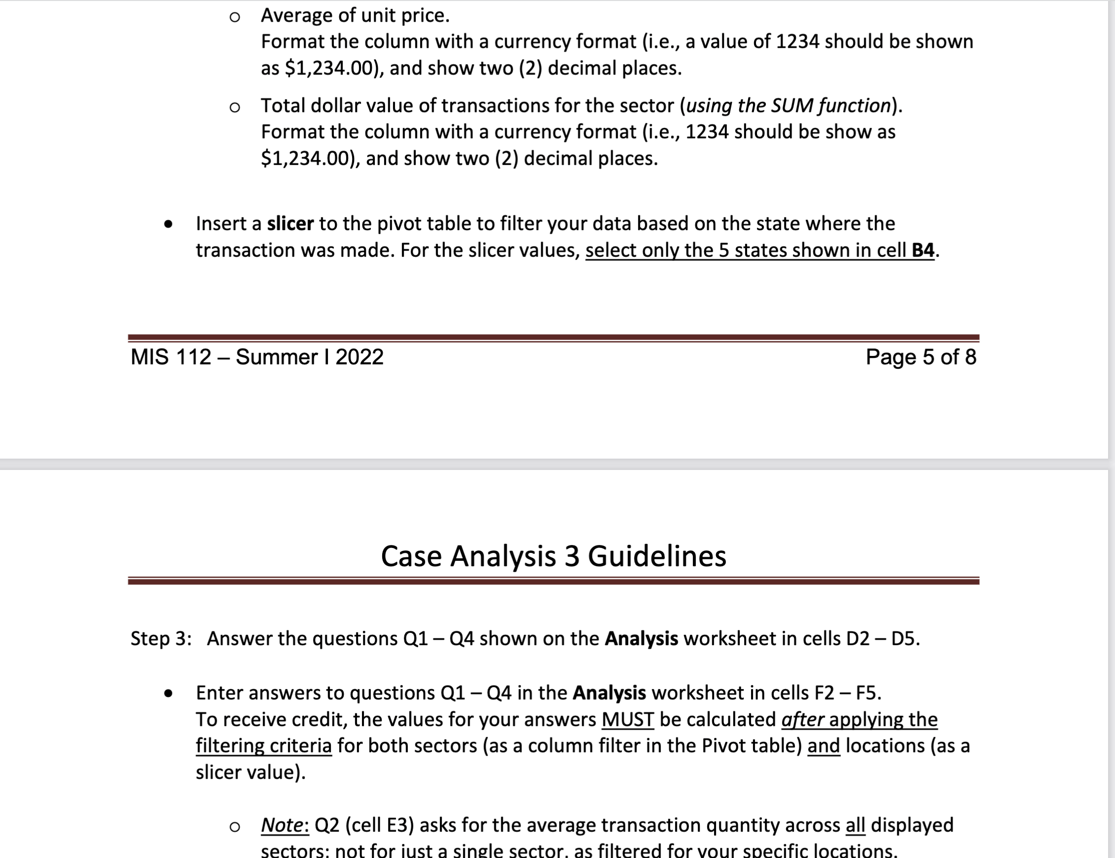
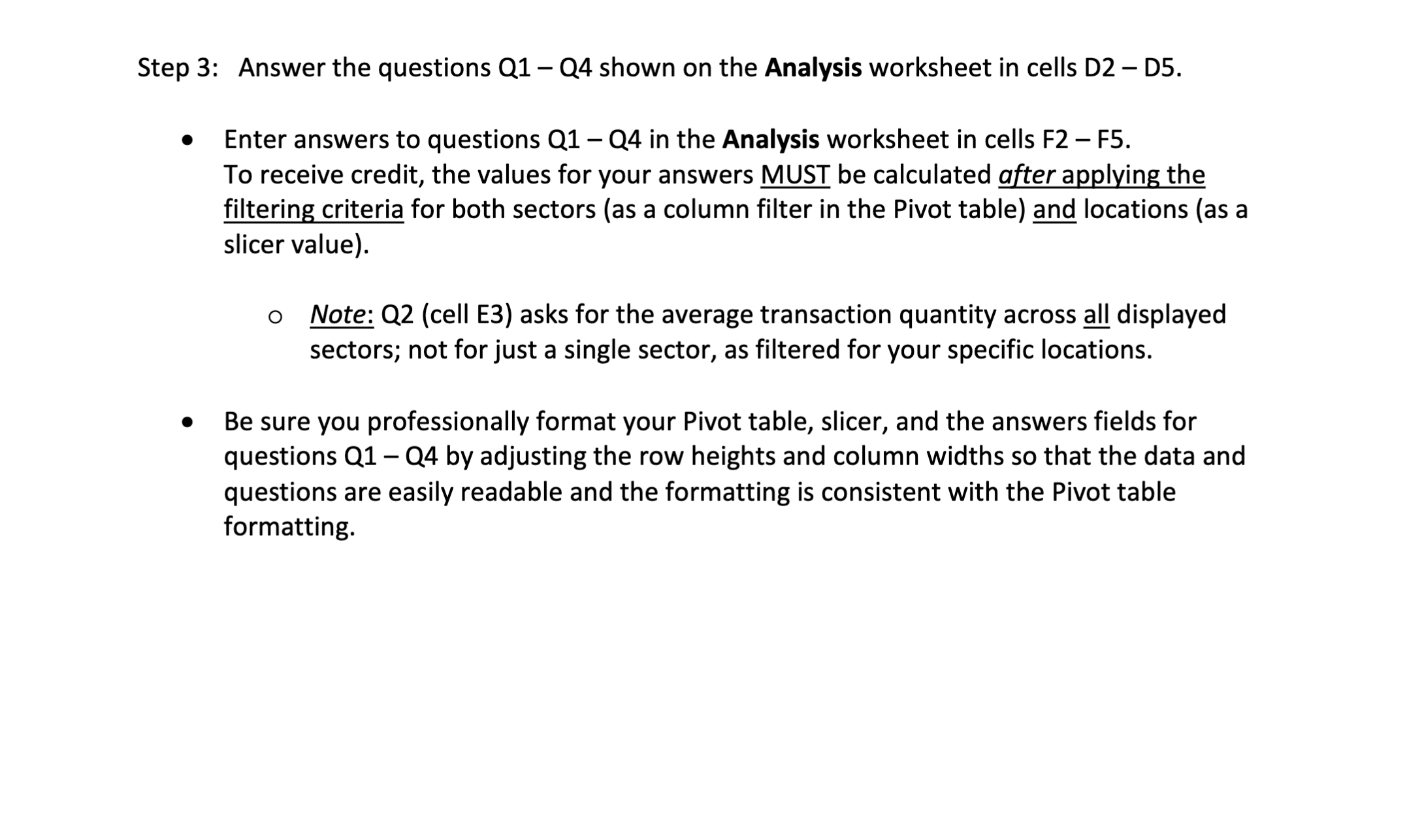
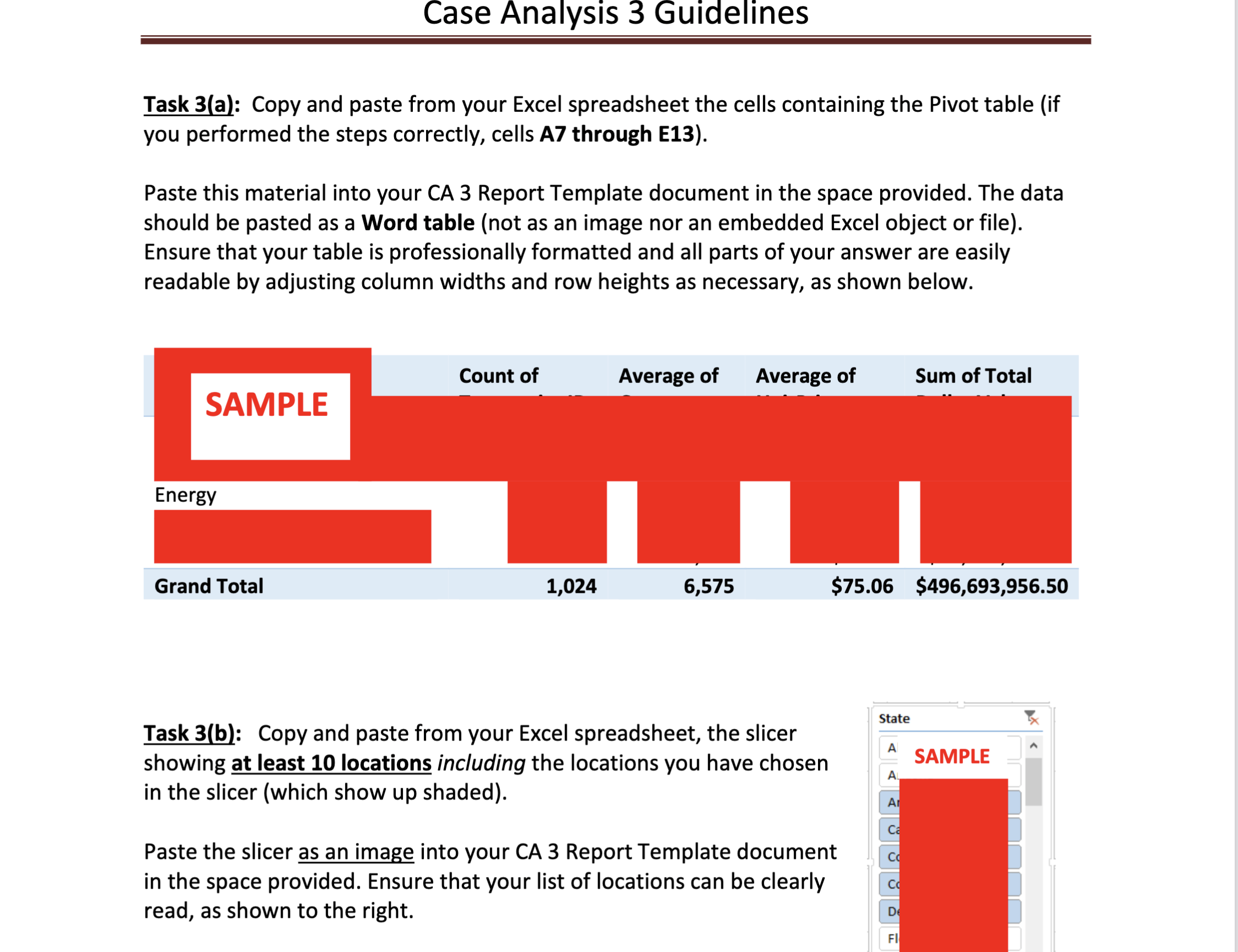
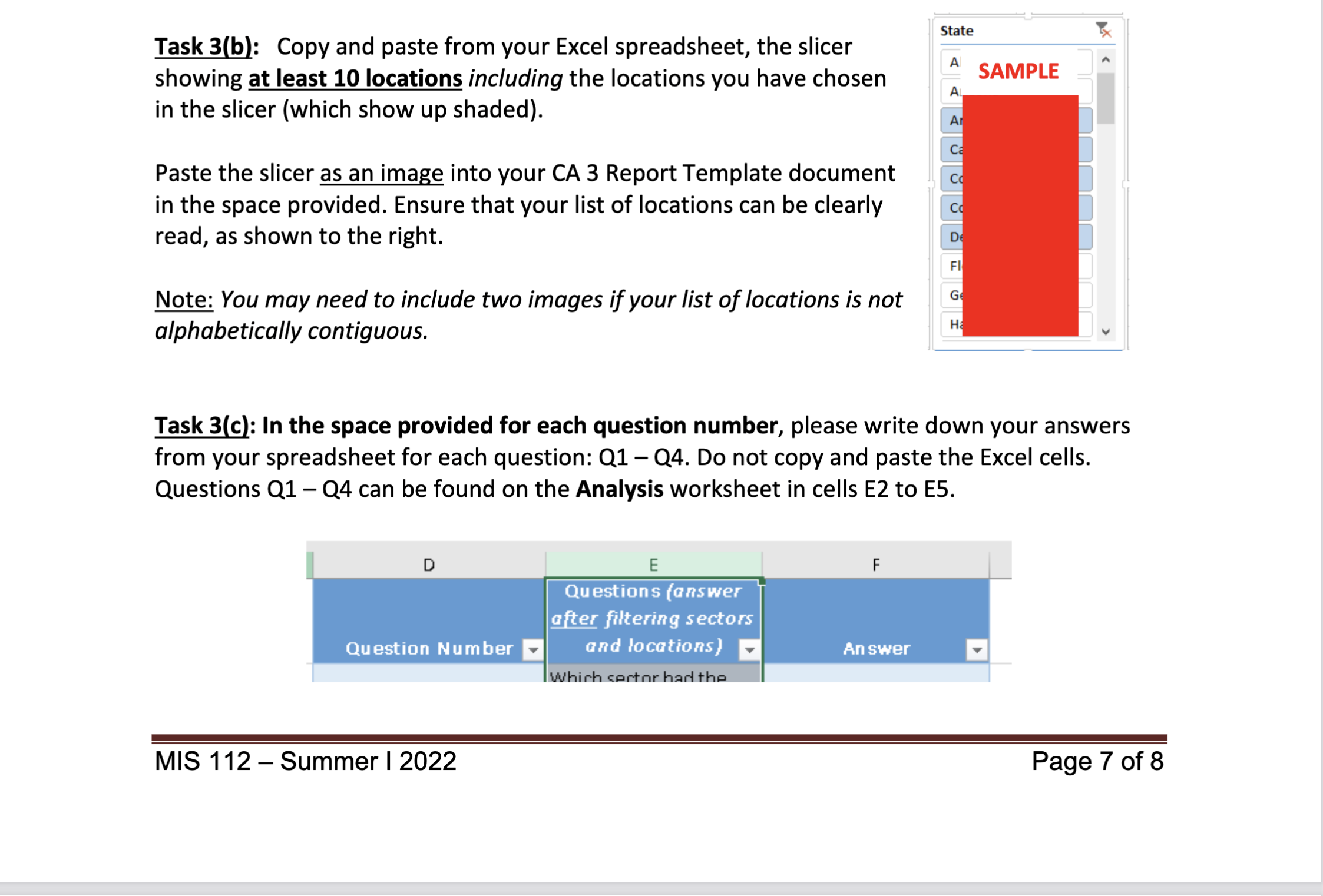
Task 3 Pivot table Follow the directions shown below to prepare a PivotTabIe. Step 1: Insert a new Pivot table in the Analysis worksheet using the \"Pivot Table\" function on the \"Insert\" ribbon, as follows: 0 Select cell A7 in the Analysis worksheet - Insert a PivotTable based on the (entire) table of data in the RawData worksheet o The new Pivot table should appear on the Analysis worksheet. Step 2: Populate the Pivot table, as follows: 0 In the PivotTables Fields pane, drag-and-drop the Sector field into the ROWS area. 0 On the Pivot table, change the column heading from Row Labels to Sector. 0 On the Pivot table, use the drop-down menu to filter the column, so that only the sector types shown in cell B_3 are selected (i.e., corresponding to the Sector filter). 0 In the PivotTables Fields pane, create the following four items in the VALUES area (by dragging-and-d ropping the appropriate fields into the VALUES area). They will later be used to answer questions 01-04. 0 Number of unique transactions (using the COUNTfunction). Format the column with a comma separating the thousands value (Le, \"7654" would be displayed as \"7,654\"), and do not include any decimal places (i.e., "4567\" would be displayed as \"4,567\" and n_ot \"4567.00\") 0 Average of quantity purchased per transaction. Format the column with a \0 Average of unit price. Format the column with a currency format (i.e., a value of 1234 should be shown as $1,234.00), and show two (2) decimal places. 0 Total dollar value of transactions for the sector (using the SUM function). Format the column with a currency format (i.e., 1234 should be show as $1,234.00), and show two (2) decimal places. 0 Insert a slicer to the pivot table to filter your data based on the state where the transaction was made. For the slicer values, select only the 5 states shown in cell B4. MIS 112 Summer | 2022 Page 5 of 8 Case Analysis 3 Guidelines Step 3: Answer the questions Ql Q4 shown on the Analysis worksheet in cells D2 DS. 0 Enter answers to questions Q1 Q4 in the Analysis worksheet in cells F2 F5. To receive credit, the values for your answers MUST be calculated after applying the filtering criteria for both sectors (as a column filter in the Pivot table) locations (as a slicer value). 0 Note: (12 (cell E3) asks for the average transaction quantity across a_H displayed sectors: not for iust a single sector. as filtered for vour specific locations. Step 3: Answer the questions Q1 Q4 shown on the Analysis worksheet in cells D2 DS. 0 Enter answers to questions Q1 - Q4 in the Analysis worksheet in cells F2 F5. To receive credit, the values for your answers MUST be calculated after applying the filtering criteria for both sectors (as a column filter in the Pivot table) locations (as a slicer value). 0 Note: Q2 (cell E3) asks for the average transaction quantity across a_|| displayed sectors; not for just a single sector, as filtered for your specific locations. 0 Be sure you professionally format your Pivot table, slicer, and the answers fields for questions (11 Q4 by adjusting the row heights and column widths so that the data and questions are easily readable and the formatting is consistent with the Pivot table formatting. Case Analysis 3 Guidelines Task 3(al: Copy and paste from your Excel spreadsheet the cells containing the Pivot table (if you performed the steps correctly, cells A7 through E13). Paste this material into your CA 3 Report Template document in the space provided. The data should be pasted as a Word table (not as an image nor an embedded Excel object or file). Ensure that your table is professionally formatted and all parts of your answer are easily readable by adjusting column widths and row heights as necessary, as shown below. Count of Sum of Total Average of Average of Energy Grand Total 1,024 6,575 $75.06 $496,693,956.50 state 7x Task 31b}: Copy and paste from your Excel spreadsheet, the slicer A showing at least 10 locations including the locations you have chosen A SAMPLE in the slicer (which show up shaded). Paste the slicer as an image into your CA 3 Report Template document in the space provided. Ensure that your list of locations can be clearly read, as shown to the right. Task 3lbl: Copy and paste from your Excel spreadsheet, the slicer showing at least 10 locations including the locations you have chosen in the slicer (which show up shaded). Paste the slicer as an image into your CA 3 Report Template document in the space provided. Ensure that your list of locations can be clearly read, as shown to the right. Note: You may need to include two images if your list of locations is not alphabetical/y contiguous. state A A SAMPLE Task 3M: In the space provided for each question number, please write down your answers from your spreadsheet for each question: Q1 Q4. Do not copy and paste the Excel cells. Questions Q1 Q4 can be found on the Analysis worksheet in cells E2 to E5. Questions (answeir aer filtering sectors Question Number and locations) MIS 112 Summer | 2022 Page 7 of 8