Test the null hypothesis (against the two-sided alternative at the 5% level of sig- nificance) that ability has the same effect on educational attainment in urban and nonurban areas, after controlling for parents education.

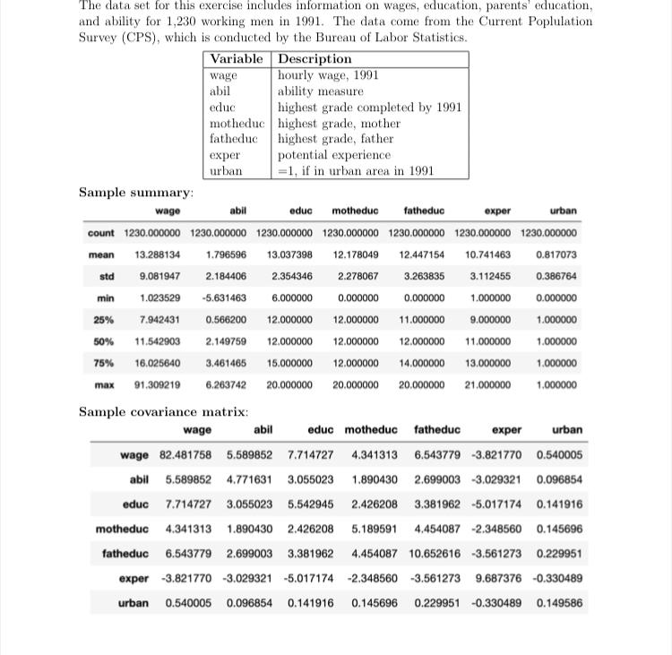
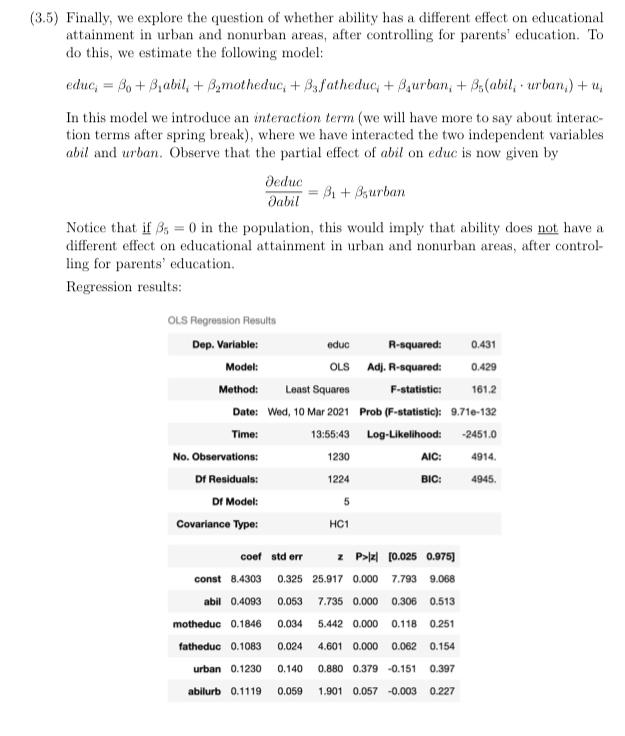
The data set for this exercise includes information on wages, education, parents' education, and ability for 1,230 working men in 1991. The data come from the Current Poplulation Survey (CPS), which is conducted by the Bureau of Labor Statistics. Variable Description wage hourly wage, 1991 abil ability measure educ highest grade completed by 1991 motheduc highest grade, mother fatheduc highest grade, father exper potential experience urban =1, if in urban area in 1991 Sample summary: wage abil educ motheduc fatheduc exper urban count 1230.000000 1230.000000 1230.000000 1230.000000 1230.000000 1230.000000 1230.000000 mean 13.288134 1.796596 13.037398 12.178049 12.447154 10.741463 0.817073 std 9.081947 2.184406 2.354346 2.278067 3.263835 3.112455 0.386764 min 1.023529 -5.631463 6.000000 0.000000 0.000000 1.000000 0.000000 25% 7.942431 0.566200 12.000000 12.000000 11.000000 9.000000 1.000000 50% 11.542903 2.149759 12.000000 12.000000 12.000000 11.000000 1.000000 75% 16.025640 3.461465 15.000000 12.000000 14.000000 13.000000 1.000000 max 91.309219 6.263742 20.000000 20.000000 20.000000 21.000000 1.000000 Sample covariance matrix wage educ motheduc fatheduc exper urban wage 82.481758 5.589852 7.714727 4.341313 6.543779 -3.821770 0.540005 abil 5.589852 4.771631 3.055023 1.890430 2.699003 -3.029321 0.096854 educ 7.7147273.055023 5.542945 2.426208 3.381962 -5.017174 0.141916 motheduc 4.341313 1.890430 2.426208 5.189591 4.454087 -2.348560 0.145696 fatheduc 6.543779 2.699003 3.381962 4.454087 10.652616 -3.561273 0.229951 exper-3.821770 -3.029321 -5.017174 -2.348560 -3.561273 9.687376 -0.330489 urban 0.540005 0.096854 0.141916 0.145696 0.229951 -0.330489 0.149586 abil (3.5) Finally, we explore the question of whether ability has a different effect on educational attainment in urban and nonurban areas, after controlling for parents' education. To do this, we estimate the following model: educ, = B. + , abil, + B, motheduc, +33 fatheduc + Saurban, + Ba(abil, urban.) + u. In this model we introduce an interaction term (we will have more to say about interac- tion terms after spring break), where we have interacted the two independent variables abil and urban. Observe that the partial effect of abil on educ is now given by Deduc dabil B1 + Asurban Notice that if B5 = 0 in the population, this would imply that ability does not have a different effect on educational attainment in urban and nonurban areas, after control- ling for parents' education. Regression results: 1224 OLS Regression Results Dep. Variable: educ R-squared: 0.431 Model: OLS Adj. R-squared: 0.429 Method: Least Squares F-statistic 161.2 Date: Wed, 10 Mar 2021 Prob (F-statistic): 9.710-132 Time: 13:55:43 Log-Likelihood: -2451.0 No. Observations: 1230 AIC: 4914 Dr Residuals: BIC: 4945 Di Model: 5 Covariance Type: HC1 coef std err z (0.025 0.975) const 8.4303 0.325 25.917 0.000 7.793 9.068 0.053 7.735 0.000 0.306 0.513 motheduc 0.1846 0.034 5.442 0.000 0.118 0.251 fatheduc 0.1083 0.024 4.601 0.000 0.062 0.154 0.140 0.880 0.379 -0.151 0.397 abil 0.4093 urban 0.1230 abilurb 0.1119 0.059 1.901 0.057 -0.003 0.227 The data set for this exercise includes information on wages, education, parents' education, and ability for 1,230 working men in 1991. The data come from the Current Poplulation Survey (CPS), which is conducted by the Bureau of Labor Statistics. Variable Description wage hourly wage, 1991 abil ability measure educ highest grade completed by 1991 motheduc highest grade, mother fatheduc highest grade, father exper potential experience urban =1, if in urban area in 1991 Sample summary: wage abil educ motheduc fatheduc exper urban count 1230.000000 1230.000000 1230.000000 1230.000000 1230.000000 1230.000000 1230.000000 mean 13.288134 1.796596 13.037398 12.178049 12.447154 10.741463 0.817073 std 9.081947 2.184406 2.354346 2.278067 3.263835 3.112455 0.386764 min 1.023529 -5.631463 6.000000 0.000000 0.000000 1.000000 0.000000 25% 7.942431 0.566200 12.000000 12.000000 11.000000 9.000000 1.000000 50% 11.542903 2.149759 12.000000 12.000000 12.000000 11.000000 1.000000 75% 16.025640 3.461465 15.000000 12.000000 14.000000 13.000000 1.000000 max 91.309219 6.263742 20.000000 20.000000 20.000000 21.000000 1.000000 Sample covariance matrix wage educ motheduc fatheduc exper urban wage 82.481758 5.589852 7.714727 4.341313 6.543779 -3.821770 0.540005 abil 5.589852 4.771631 3.055023 1.890430 2.699003 -3.029321 0.096854 educ 7.7147273.055023 5.542945 2.426208 3.381962 -5.017174 0.141916 motheduc 4.341313 1.890430 2.426208 5.189591 4.454087 -2.348560 0.145696 fatheduc 6.543779 2.699003 3.381962 4.454087 10.652616 -3.561273 0.229951 exper-3.821770 -3.029321 -5.017174 -2.348560 -3.561273 9.687376 -0.330489 urban 0.540005 0.096854 0.141916 0.145696 0.229951 -0.330489 0.149586 abil (3.5) Finally, we explore the question of whether ability has a different effect on educational attainment in urban and nonurban areas, after controlling for parents' education. To do this, we estimate the following model: educ, = B. + , abil, + B, motheduc, +33 fatheduc + Saurban, + Ba(abil, urban.) + u. In this model we introduce an interaction term (we will have more to say about interac- tion terms after spring break), where we have interacted the two independent variables abil and urban. Observe that the partial effect of abil on educ is now given by Deduc dabil B1 + Asurban Notice that if B5 = 0 in the population, this would imply that ability does not have a different effect on educational attainment in urban and nonurban areas, after control- ling for parents' education. Regression results: 1224 OLS Regression Results Dep. Variable: educ R-squared: 0.431 Model: OLS Adj. R-squared: 0.429 Method: Least Squares F-statistic 161.2 Date: Wed, 10 Mar 2021 Prob (F-statistic): 9.710-132 Time: 13:55:43 Log-Likelihood: -2451.0 No. Observations: 1230 AIC: 4914 Dr Residuals: BIC: 4945 Di Model: 5 Covariance Type: HC1 coef std err z (0.025 0.975) const 8.4303 0.325 25.917 0.000 7.793 9.068 0.053 7.735 0.000 0.306 0.513 motheduc 0.1846 0.034 5.442 0.000 0.118 0.251 fatheduc 0.1083 0.024 4.601 0.000 0.062 0.154 0.140 0.880 0.379 -0.151 0.397 abil 0.4093 urban 0.1230 abilurb 0.1119 0.059 1.901 0.057 -0.003 0.227