...Thanks.

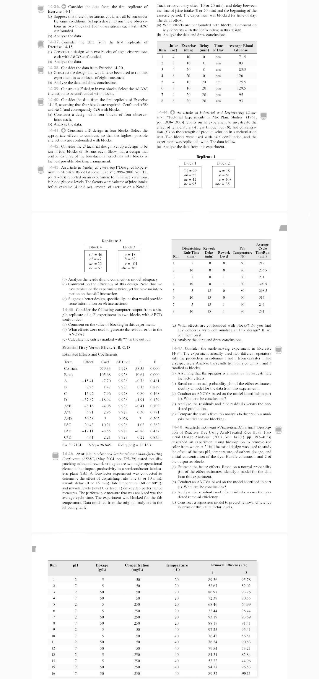
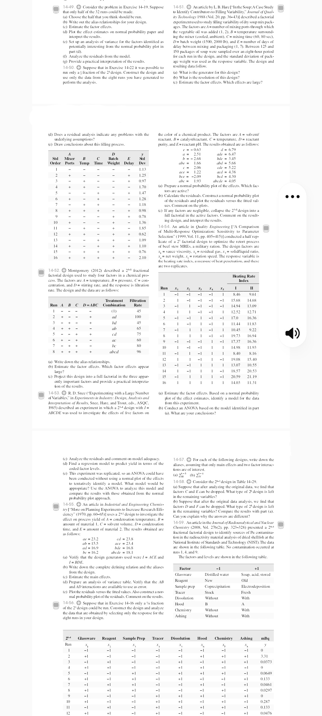
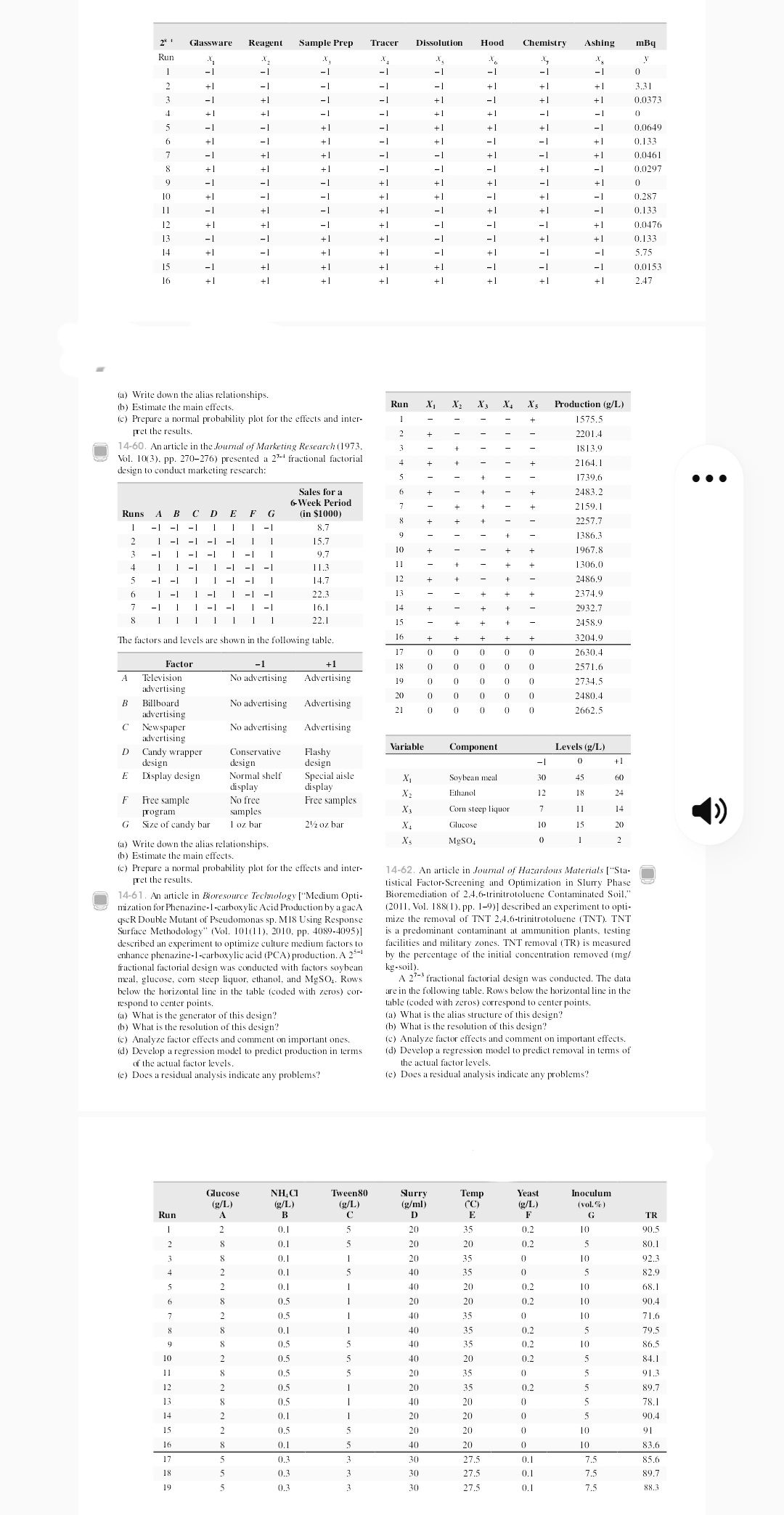
14-36. + Consider the data from the first replicate of Track cross-country skier (10 or 20 min), and delay between Exercise 14-14. the time of juice intake (0 or 20 min) and the beginning of the (a) Suppose that these observations could not all be run under exercise period. The experiment was blocked for time of day. the same conditions. Set up a design to run these observa- The data follow. tions in two blocks of four observations each with ABC (a) What effects are confounded with blocks? Comment on confounded. any concerns with the confounding in this design. (b) Analyze the data. (b) Analyze the data and draw conclusions. 14-37. Consider the data from the first replicate of Exercise 14-15. Juice Exercise Delay Time Average Blood (a) Construct a design with two blocks of eight observations Run (oz) (min) (min) of Day Glucose cach with ABCD confounded. pm 71.5 (b) Analyze the data. 103 14-38. Consider the data from Exercise 14-20. 20 0 am 83.5 (a) Construct the design that would have been used to run this experiment in two blocks of eight runs each. 20 pm 126 (b) Analyze the data and draw conclusions. 10 20 125. 14-39. Construct a 2' design in two blocks. Select the ABCDE 10 20 pm 129.5 interaction to be confounded with blocks. 20 20 pm 95 14-40. Consider the data from the first replicate of Exercise 8 8 20 20 am 03 14-15, assuming that four blocks are required. Confound ABD and ABC (and consequently CD) with blocks. a) Construct a design with four blocks of four observa- 14-44. + An article in Industrial and Engineering Chem- tions cach. istry ["Factorial Experiments in Pilot Plant Studies" (1951. (b) Analyze the data. pp. 1300-1306)] reports on an experiment to investigate the 14-41. + Construct a 2' design in four blocks. Select the effect of temperature (A), gas throughput (B), and concentra- tion (C) on the strength of product solution in a recirculation appropriate effects to confound so that the highest possible unit. Two blocks were used with ABC confounded, and the interactions are confounded with blocks. experiment was replicated twice. The data follow. 14-42. Consider the 2% factorial design. Set up a design to be (a) Analyze the data from this experiment run in four blocks of 16 runs each. Show that a design that confounds three of the four-factor interactions with blocks is Replicate 1 the best possible blocking arrangement. Block I Block 2 14-43. An article in Quality Engineering ["Designed Experi- ment to Stabilize Blood Glucose Levels" (1999-2000, Vol. 12 (1) =99 a = 18 pp. 83-87)1 reported on an experiment to minimize variations ab = 52 b = 51 in blood glucose levels. The factors were volume of juice intake ac = 42 C = 108 be = 95 abc = 35 before exercise (4 or 8 oz), amount of exercise on a Nordic Replicate 2 Block 4 Block 3 Average Dispatching Rework Fab Cycle (1) = 46 Rule Time a = 18 Delay Rework Temperature TimeRun (min) (min) Level ('F) ab = 47 b = 62 Run (min) ac = 22 c = 104 60 218 bc = 67 ibc = 36 80 256.5 80 231 (b) Analyze the residuals and comment on model adequacy. c) Comment on the efficiency of this design. Note that we 10 60 302.5 have replicated the experiment twice, yet we have no infor- 15 80 298.5 mation on the ABC interaction. d) Suggest a better design, specifically one that would provide 10 60 314 some information on all interactions. 15 60 249 14-45. Consider the following computer output from a sin- 10 15 gle replicate of a 2" experiment in two blocks with ABCD confounded. (a) Comment on the value of blocking in this experiment. (a) What effects are confounded with blocks? Do you find (b) What effects were used to generate the residual error in the any concerns with confounding in this design? If so. ANOVA? comment on it. (c) Calculate the entries marked with "?" in the output. (b) Analyze the darta and draw conclusions. Factorial Fit: y Versus Block, A, B, C, D 14-47. Consider the earth-moving experiment in Exercise Estimated Effects and Coefficients 14-34. The experiment actually used two different operators with the production in columns I and 3 from operator I and Term Effect Coef SE Coef P 2, respectively. Analyze the results from only columns I and 3 Constant 579.33 9.928 58.35 0.000 bundled as blocks. Block 105.68 9.928 10.64 0.000 a) Assuming that the operator is a nui e factor, estimate the factor effects. A -15.41 -7.70 9,928 -0.78 0.481 b) Based on a normal probability plot of the effect estimates. B 2.95 1.47 9.928 0.15 0.889 identify a model for the data from this experiment. 15.9 796 9.928 0.80 0.468 ") Conduct an ANOVA based on the model identified in part D -37.87 -18.94 9.928 -1.91 0.129 (a). What are the conclusions? -8.16 -4.08 9.928 -0.41 0.702 d) Analyze the residuals and plot residuals versus the pre- acted production. A*C 5.91 95 9.928 0.30 0.781 (e) Compare the results from this analysis to the previous anal- A*D 30.28 ).202 ysis that did not use blocking. B*C 20.43 10.21 1928 103 0.362 14-48. An article in Journal of Hazardous Materials ["Biosorp- B*D -17.11 -8.55 9.928 -0.86 0.437 tion of Reactive Dye Using Acid-Treated Rice Husk: Fac- C*D 4.41 2.21 9.928 0.22 0.835 torial Design Analysis" (2007, Vol. 142(1), pp. 397-403)1 S = 39.7131 R-Sq = 96.84% R-Sq (adj) = 88.16% described an experiment using biosorption to remove red color from water. A 2" full factorial design was used to study 14-46. An article in Advanced Semiconductor Manufacturing the effect of factors pH. temperature, adsorbent dosage, and Conference (ASMC) (May 2004. pp. 325-29) stated that dis- initial concentration of the dye. Handle columns I and 2 of patching rules and rework strategies are two major operational the output as blocks. elements that impact productivity in a semiconductor fabrica- (a) Estimate the factor effects. Based on a normal probability tion plant (fab). A four-factor experiment was conducted to plot of the effect estimates, identify a model for the data determine the effect of dispatching rule time (5 or 10 min). from this experiment. rework delay (0 or 15 min), fab temperature (60 or 80 F). (b) Conduct an ANOVA based on the model identified in part and rework levels (level 0 or level 1) on key fab performance (a). What are the conclusions? measures. The performance measure that was analyzed was the (c) Analyze the residuals and plot residuals versus the pre- average cycle time. The experiment was blocked for the fab dicted removal efficiency. temperature. Data modified from the original study are in the (d) Construct a regression model to predict removal efficiency following table. in terms of the actual factor levels. Run PH Dosage Concentration Temperature Removal Efficiency ("%) (g/L) (mg/L) (C) 20 89.36 95.78 IN 20 53.67 52.02 20 86.97 93.76 20 72 39 80.55 250 20 68.4 64.99 250 20 32.44 28.44 250 20 93.19 93.69 250 20 88.17 91.41 50 40 97.25 95.41 40 76.42 56.51 40 76.24 90.83 40 79.54 73.21 40 84.31 82.84 40 53.32 44.96 40 94.77 96.53 89.32 90.7514-49. + Consider the problem in Exercise 14-19. Suppose 14-51. + An article by L. B. Hare ["In the Soup:A Case Study that only half of the 32 runs could be made. Identify Contributors to Filling Variability." Journal of Qual- a) Choose the half that you think should be run. ity Technology 1988 (Vol. 20. pp. 36-43)] described a factorial (b) Write out the alias relationships for your design. experiment used to study filling variability of dry soup mix pack- (c) Estimate the factor effects. ages. The factors are A = number of mixing ports through which d) Plot the effect estimates on normal probability paper and the vegetable oil was added (1. 2). B = temperature surround- interpret the results. ing the mixer (cooled, ambient). C= mixing time (60, 80 sec). (e) Set up an analysis of variance for the factors identified as D= batch weight (1500, 2000 1b), and E = number of days of potentially interesting from the normal probability plot in delay between mixing and packaging (1. 7). Between 125 and part (d). 150 packages of soup were sampled over an eight-hour period f) Analyze the residuals from the model. for each run in the design, and the standard deviation of pack- (@) Provide a practical interpretation of the results. age weight was used as the response variable. The design and 14-50. + Suppose that in Exercise 14-22 it was possible to resulting data follow. run only a : fraction of the 24 design. Construct the design and (a) What is the generator for this design? use only the data from the eight runs you have generated to (b) What is the resolution of this design? perform the analysis. (c) Estimate the factor effects. Which effects are large? (d) Does a residual analysis indicate any problems with the the color of a chemical product. The factors are A = solvent/ underlying assumptions? reactant, B = catalyst/reactant, C = temperature, D = reactant (e) Draw conclusions about this filling process. purity. and E= reactant pH. The results obtained are as follows: e = - 0.63 d = 6.79 2.51 ade = 6.47 Std Mixer B C Batch E Sid b = - 2.68 bde = 3.45 Order Ports Temp Time Weight Delay Dev abe = 1.66 abd = 5.68 1.13 2.06 cde = 5.22 ace = 1.22 acd = 4.38 1.25 = -2.09 bed = 4.30 0.97 abc = 1.93 abcde = 4.05 1.70 (@) Prepare a normal probability plot of the effects. Which fac- 1.47 tors are active? b) Calculate the residuals. Construct a normal probability plot 1.28 . . . of the residuals and plot the residuals versus the fitted val- 1. 18 ucs. Comment on the plots. 0.98 (c) If any factors are negligible, collapse the 2"- design into a 0.7 full factorial in the active factors. Comment on the result- 10 1.36 ing design, and interpret the results. 1.85 14-54. An article in Quality Engineering ["A Comparison 0.62 of Multi-Response Optimization: Sensitivity to Parameter Selection" (1999, Vol. 1 1, pp. 405-415) | conducted a half rep- 1.09 licate of a 2' factorial design to optimize the retort process 14 1.10 of beef stew MREs, a military ration. The design factors are 15 0.76 x, = sauce viscosity, x, = residual gas, x, = solid/liquid ratio. 2.10 v, = net weight. x, = rotation speed. The response variable is he beating tate index, a measure of beat penetration, and there are two replicates 14-52. + Montgomery (2012) described a 2+ fractional factorial design used to study four factors in a chemical pro- Heating Rate cess. The factors are A = temperature, B = pressure, C = con- Index centration, and D = stirring rate, and the response is filtration rate. The design and the data are as follows: Run X's 8.46 9.61 Treatment Filtration -1 15.68 14.68 Run A B C D=ABC Combination Rate 14.94 13.09 4 12.52 12.71 100 17.0 16.36 bd 11.44 11.83 ab 65 10.45 922 ed 75 19.73 16.94 ac 60 17.37 16.36 be 80 10 14.98 1193 abed 06 11 8.40 8.16 12 -1 19.08 IS.40 (a) Write down the alias relationships. b) Estimate the factor effects. Which factor effects appear 13 13.07 10.55 large? 14 -1 18.57 20.53 (c) Project this design into a full factorial in the three appar- 15 20.59 21.19 ently important factors and provide a practical interpreta- 16 14.03 11.31 tion of the results. 14-53. + R. D. Snee ("Experimenting with a Large Number (a) Estimate the factor effects. Based on a normal probability of Variables," in Experiments in Industry: Design, Analysis and plot of the effect estimates, identify a model for the data Interpretation of Results, Snee, Hare, and Trout, eds., ASQC. from this experiment. 1985) described an experiment in which a 25- design with / = b) Conduct an ANOVA based on the model identified in part ABCDE was used to investigate the effects of five factors on (a). What are your conclusions? (c) Analyze the residuals and comment on model adequacy. 14-57. + For each of the following designs, write down the d) Find a regression model to predict yield in terms of the aliases, assuming that only main effects and two factor interac- coded factor levels. tions are of interest. (e) This experiment was replicated, so an ANOVA could have (@) 217 (b) 2iv* been conducted without using a normal plot of the effects to tentatively identify a model. What model would be 14-58. + Consider the 26-2 design in Table 14-29. appropriate? Use the ANOVA to analyze this model and (a) Suppose that after analyzing the original data, we find that compare the results with those obtained from the normal factors C and E can be dropped. What type of 24 design is left probability plot approach. in the remaining variables? 14-55. + An article in Industrial and Engineering Chemis- (b) Suppose that after the original data analysis, we find that factors D and F can be dropped. What type of 24 design is left try ["More on Planning Experiments to Increase Research Effi- ciency" (1970. pp. 60-65)] uses a 232 design to investigate the in the remaining variables? Compare the results with part (a). Can you explain why the answers are different? effect on process yield of A = condensation temperature, B = amount of material 1. C = solvent volume, D = condensation 14-59. An article in the Journal of Radioanalytical and Nuclear time, and E = amount of material 2. The results obtained are Chemistry (2008. Vol. 276(2). pp. 323-328) presented a 28-4 as follows: fractional factorial design to identify sources of Pu contamina- de = 23.2 cd = 23.8 tion in the radioactivity material analysis of dried shellfish at the ab = 15.5 ace = 23.4 National Institute of Standards and Technology (NIST). The data ad = 16.9 bde = 16.8 are shown in the following table. No contamination occurred at be = 16.2 abcde = 18.1 uns 1. 4. and 9. fy that the design generators used were / = ACE and The factors and levels are shown in the following table. 1 = BDE. (b) Write down the complete defining relation and the aliases Factor +1 from the design. (c) Estimate the main effects Glassware Distilled water Soap, acid, stored (d) Prepare an analysis of variance table. Verify that the AB Reagent New Old and AD interactions are available to use as error. Sample prep Coprecipitation Electrodeposition (e) Plot the residuals versus the fitted values. Also construct a nor- Tracer Stock Fresh mal probability plot of the residuals. Comment on the results. Dissolution Without With 14-56. + Suppose that in Exercise 14-16 only a 4 fraction Hood 3 A of the 2' design could be run. Construct the design and analyze Without With the data that are obtained by selecting only the response for the Chemistry eight runs in your design. Ashing Without With Glassware Reagent Sample Prep Tracer Dissolution Hood Chemistry Ashing mBq Run 3.31 0.0373 0 +1 0.064 0.13 0.0461 0.0297 0.287 0.133 0.04762" ' Glassware Reagent Sample Prep Tracer Dissolution Hood Chemistry Ashing mBq Run 3,31 0.0373 0.0649 0.133 0.0461 0.0297 0.287 0.13. 0.0476 0.133 5.75 0.0153 2.47 (a) Write down the alias relationships. b) Estimate the main effects. Run As X4 X's Production (g/L) (c) Prepare a normal probability plot for the effects and inter- 1575.5 pret the results. 2201.4 14-60. An article in the Journal of Marketing Research (1973. 1813. vol. 10(3). pp. 270-276) presented a 23- fractional factorial 2164.1 design to conduct marketing research: 1739.6 . . . Sales for a 2483.2 Week Period Runs 2159.1 A (in $1000) 2257.7 8.7 1386.3 15.7 97 1967.8 VIAWN 11.3 1306.0 14.7 2486.9 22.3 13 2374.9 16.1 14 2932.7 22.1 15 2458.9 The factors and levels are shown in the following table. 3204.9 17 0 2630.4 Factor -1 +1 0 2571.6 Television No advertising Advertising 0 2734.5 advertising 20 0 0 0 2480.4 B Billboard No advertising Advertising 21 advertising 2662.5 Newspaper No advertising Advertising advertising D Candy wrapper Conservative Flashy Variable Component Levels (g/L) design design design 0 E Display design Normal shelf Special aisle Soybean meal 45 60 display display X2 Ethanol 18 24 F Free sample No free Free samples program samples X 1 Corn steep liquor 14 ()) G Size of candy bar I oz bar 21/2 oz bar XA Glucose 10 15 20 a) Write down the alias relationships. MeSO (b) Estimate the main effects. c) Prepare a normal probability plot for the effects and inter- 14-62. An article in Journal of Hazardous Materials ["Sta- pret the results. tistical Factor-Screening and Optimization in Slurry Phase 14-61. An article in Broresource Technology ["Medium Opti- Bioremediation of 2.4.6-trinitrotoluene Contaminated Soil." mization for Phenazine-I-carboxylic Acid Production by a gacA (2011, Vol. 188(1), pp. 1-9)1 described an experiment to opti- qscR Double Mutant of Pseudomonas sp. M18 Using Response mize the removal of TNT 2.4.6-trinitrotoluene (TNT). TNT Surface Methodology" (Vol. 101 (11). 2010, pp. 4089-4095)] is a predominant contaminant at ammunition plants, testing described an experiment to optimize culture medium factors to facilities and military zones. TNT removal (TR) is measured enhance phenazine-I-carboxylic acid (PCA) production. A 25-1 by the percentage of the initial concentration removed (mg/ fractional factorial design was conducted with factors soybean