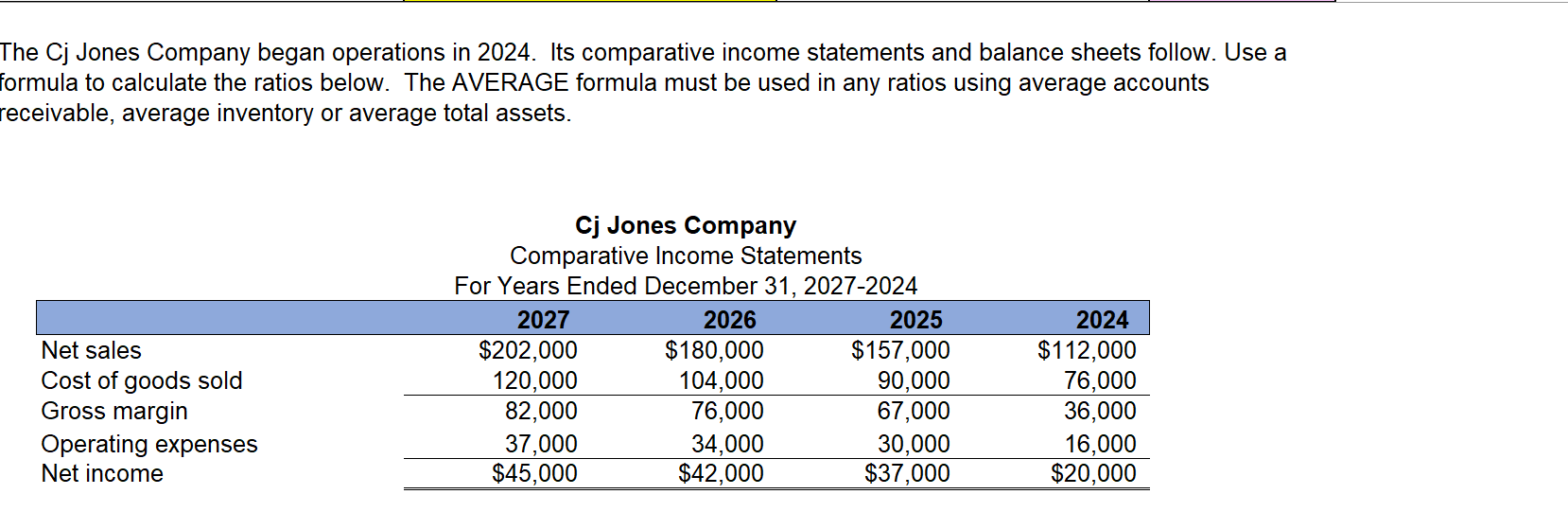
The Cj Jones Company began operations in 2024. Its comparative income statements and balance sheets follow....

Transcribed Image Text:

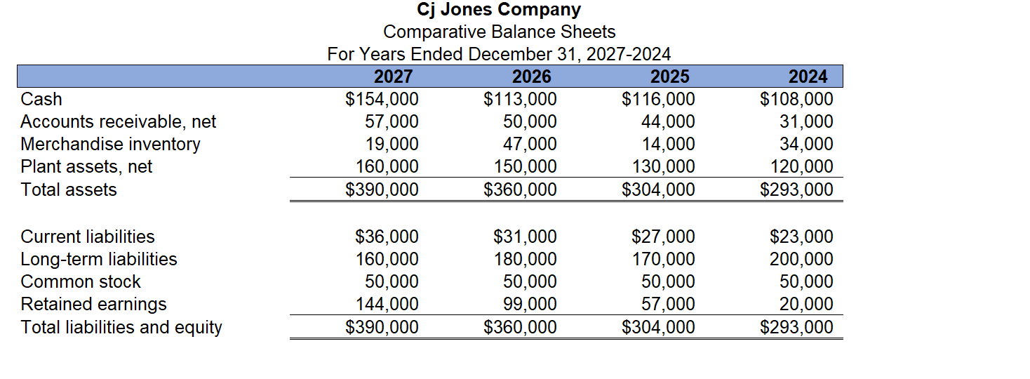
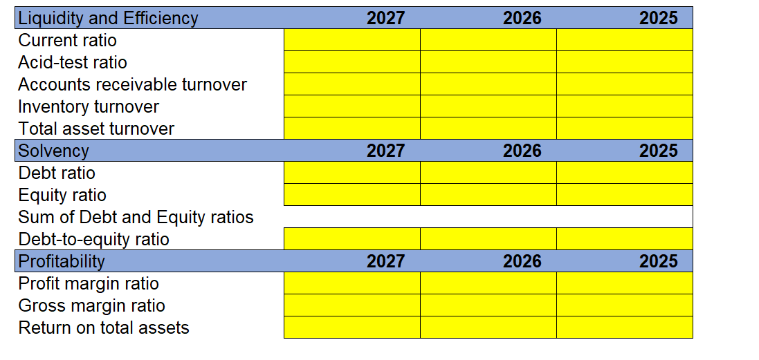
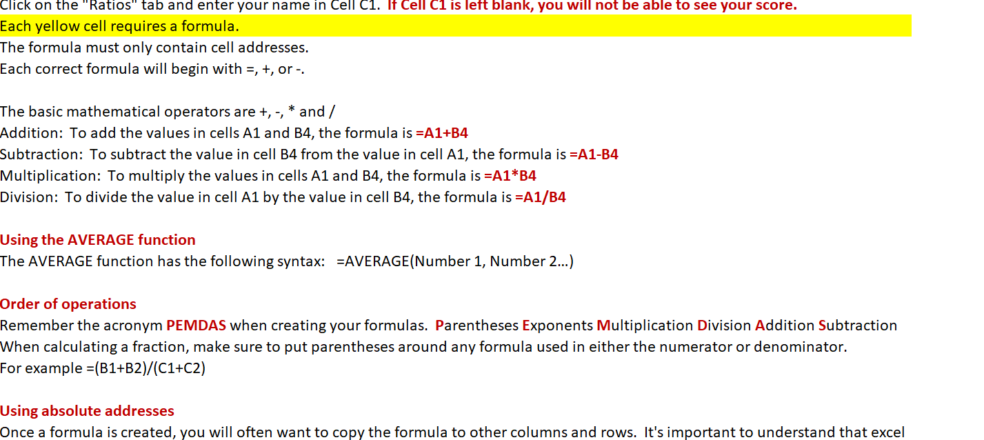
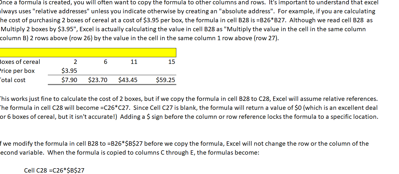
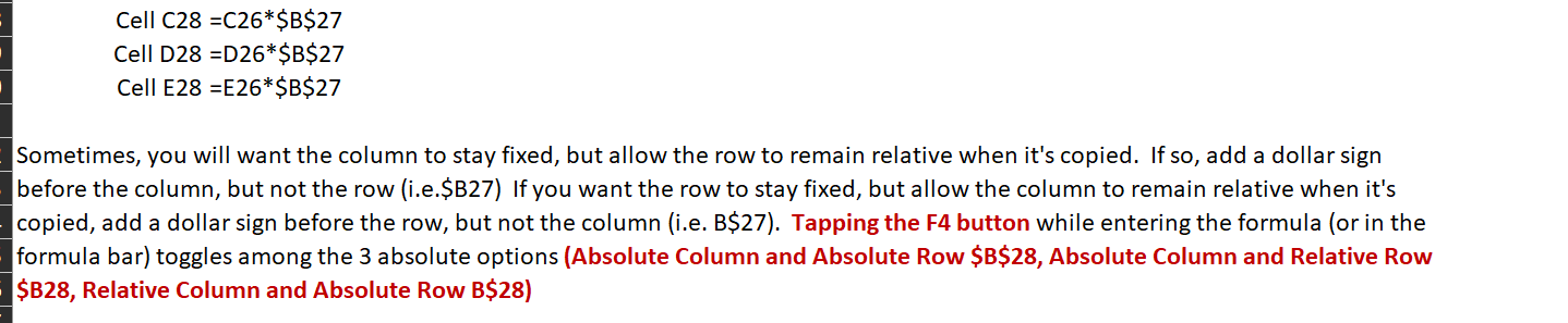
The Cj Jones Company began operations in 2024. Its comparative income statements and balance sheets follow. Use a formula to calculate the ratios below. The AVERAGE formula must be used any ratios using average accounts receivable, average inventory or average total assets. Net sales Cost of goods sold Gross margin Operating expenses Net income Cj Jones Company Comparative Income Statements For Years Ended December 31, 2027-2024 2027 $202,000 120,000 82,000 37,000 $45,000 2026 $180,000 104,000 76,000 34,000 $42,000 2025 $157,000 90,000 67,000 30,000 $37,000 2024 $112,000 76,000 36,000 16,000 $20,000 Cash Accounts receivable, net Merchandise inventory Plant assets, net Total assets Current liabilities Long-term liabilities Common stock Retained earnings Total liabilities and equity Cj Jones Company Comparative Balance Sheets For Years Ended December 31, 2027-2024 2027 $154,000 57,000 19,000 160,000 $390,000 $36,000 160,000 50,000 144,000 $390,000 2026 $113,000 50,000 47,000 150,000 $360,000 $31,000 180,000 50,000 99,000 $360,000 2025 $116,000 44,000 14,000 130,000 $304,000 $27,000 170,000 50,000 57,000 $304,000 2024 $108,000 31,000 34,000 120,000 $293,000 $23,000 200,000 50,000 20,000 $293,000 Liquidity and Efficiency Current ratio Acid-test ratio Accounts receivable turnover Inventory turnover Total asset turnover Solvency Debt ratio Equity ratio Sum of Debt and Equity ratios Debt-to-equity ratio Profitability Profit margin ratio Gross margin ratio Return on total assets 2027 2027 2027 2026 2026 2026 2025 2025 2025 Click on the "Ratios" tab and enter your name in Cell C1. If Cell C1 is left blank, you will not be able to see your score. Each yellow cell requires a formula. The formula must only contain cell addresses. Each correct formula will begin with =, +, or -. The basic mathematical operators are +, - Addition: To add the values in cells A1 and B4, the formula is =A1+B4 * and/ Subtraction: To subtract the value in cell B4 from the value in cell A1, the formula is =A1-B4 Multiplication: To multiply the values in cells A1 and B4, the formula is =A1*B4 Division: To divide the value in cell A1 by the value in cell B4, the formula is =A1/B4 Using the AVERAGE function The AVERAGE function has the following syntax: =AVERAGE(Number 1, Number 2...) Order of operations Remember the acronym PEMDAS when creating your formulas. Parentheses Exponents Multiplication Division Addition Subtraction When calculating a fraction, make sure to put parentheses around any formula used in either the numerator or denominator. For example =(B1+B2)/(C1+C2) Using absolute addresses Once a formula is created, you will often want to copy the formula to other columns and rows. It's important to understand that excel Once a formula is created, you will often want to copy the formula to other columns and rows. It's important to understand that excel lways uses "relative addresses" unless you indicate otherwise by creating an "absolute address". For example, if you are calculating he cost of purchasing 2 boxes of cereal at a cost of $3.95 per box, the formula in cell B28 is =B26*B27. Although we read cell B28 as Multiply 2 boxes by $3.95", Excel is actually calculating the value in cell B28 as "Multiply the value in the cell in the same column column B) 2 rows above (row 26) by the value in the cell in the same column 1 row above (row 27). Boxes of cereal Price per box otal cost 2 $3.95 $7.90 6 $23.70 Cell C28 =C26*$B$27 11 $43.45 15 $59.25 his works just fine to calculate the cost of 2 boxes, but if we copy the formula in cell B28 to C28, Excel will assume relative references. The formula in cell C28 will become =C26*C27. Since Cell C27 is blank, the formula will return a value of $0 (which is an excellent deal or 6 boxes of cereal, but it isn't accurate!) Adding a $sign before the column or row reference locks the formula to a specific location. f we modify the formula in cell B28 to =B26*$B$27 before we copy the formula, Excel will not change the row or the column of the econd variable. When the formula is copied to columns C through E, the formulas become: Cell C28 =C26*$B$27 Cell D28 =D26*$B$27 Cell E28 =E26*$B$27 Sometimes, you will want the column to stay fixed, but allow the row to remain relative when it's copied. If so, add a dollar sign before the column, but not the row (i.e.$B27) If you want the row to stay fixed, but allow the column to remain relative when it's copied, add a dollar sign before the row, but not the column (i.e. B$27). Tapping the F4 button while entering the formula (or in the formula bar) toggles among the 3 absolute options (Absolute Column and Absolute Row $B$28, Absolute Column and Relative Row $B28, Relative Column and Absolute Row B$28) The Cj Jones Company began operations in 2024. Its comparative income statements and balance sheets follow. Use a formula to calculate the ratios below. The AVERAGE formula must be used any ratios using average accounts receivable, average inventory or average total assets. Net sales Cost of goods sold Gross margin Operating expenses Net income Cj Jones Company Comparative Income Statements For Years Ended December 31, 2027-2024 2027 $202,000 120,000 82,000 37,000 $45,000 2026 $180,000 104,000 76,000 34,000 $42,000 2025 $157,000 90,000 67,000 30,000 $37,000 2024 $112,000 76,000 36,000 16,000 $20,000 Cash Accounts receivable, net Merchandise inventory Plant assets, net Total assets Current liabilities Long-term liabilities Common stock Retained earnings Total liabilities and equity Cj Jones Company Comparative Balance Sheets For Years Ended December 31, 2027-2024 2027 $154,000 57,000 19,000 160,000 $390,000 $36,000 160,000 50,000 144,000 $390,000 2026 $113,000 50,000 47,000 150,000 $360,000 $31,000 180,000 50,000 99,000 $360,000 2025 $116,000 44,000 14,000 130,000 $304,000 $27,000 170,000 50,000 57,000 $304,000 2024 $108,000 31,000 34,000 120,000 $293,000 $23,000 200,000 50,000 20,000 $293,000 Liquidity and Efficiency Current ratio Acid-test ratio Accounts receivable turnover Inventory turnover Total asset turnover Solvency Debt ratio Equity ratio Sum of Debt and Equity ratios Debt-to-equity ratio Profitability Profit margin ratio Gross margin ratio Return on total assets 2027 2027 2027 2026 2026 2026 2025 2025 2025 Click on the "Ratios" tab and enter your name in Cell C1. If Cell C1 is left blank, you will not be able to see your score. Each yellow cell requires a formula. The formula must only contain cell addresses. Each correct formula will begin with =, +, or -. The basic mathematical operators are +, - Addition: To add the values in cells A1 and B4, the formula is =A1+B4 * and/ Subtraction: To subtract the value in cell B4 from the value in cell A1, the formula is =A1-B4 Multiplication: To multiply the values in cells A1 and B4, the formula is =A1*B4 Division: To divide the value in cell A1 by the value in cell B4, the formula is =A1/B4 Using the AVERAGE function The AVERAGE function has the following syntax: =AVERAGE(Number 1, Number 2...) Order of operations Remember the acronym PEMDAS when creating your formulas. Parentheses Exponents Multiplication Division Addition Subtraction When calculating a fraction, make sure to put parentheses around any formula used in either the numerator or denominator. For example =(B1+B2)/(C1+C2) Using absolute addresses Once a formula is created, you will often want to copy the formula to other columns and rows. It's important to understand that excel Once a formula is created, you will often want to copy the formula to other columns and rows. It's important to understand that excel lways uses "relative addresses" unless you indicate otherwise by creating an "absolute address". For example, if you are calculating he cost of purchasing 2 boxes of cereal at a cost of $3.95 per box, the formula in cell B28 is =B26*B27. Although we read cell B28 as Multiply 2 boxes by $3.95", Excel is actually calculating the value in cell B28 as "Multiply the value in the cell in the same column column B) 2 rows above (row 26) by the value in the cell in the same column 1 row above (row 27). Boxes of cereal Price per box otal cost 2 $3.95 $7.90 6 $23.70 Cell C28 =C26*$B$27 11 $43.45 15 $59.25 his works just fine to calculate the cost of 2 boxes, but if we copy the formula in cell B28 to C28, Excel will assume relative references. The formula in cell C28 will become =C26*C27. Since Cell C27 is blank, the formula will return a value of $0 (which is an excellent deal or 6 boxes of cereal, but it isn't accurate!) Adding a $sign before the column or row reference locks the formula to a specific location. f we modify the formula in cell B28 to =B26*$B$27 before we copy the formula, Excel will not change the row or the column of the econd variable. When the formula is copied to columns C through E, the formulas become: Cell C28 =C26*$B$27 Cell D28 =D26*$B$27 Cell E28 =E26*$B$27 Sometimes, you will want the column to stay fixed, but allow the row to remain relative when it's copied. If so, add a dollar sign before the column, but not the row (i.e.$B27) If you want the row to stay fixed, but allow the column to remain relative when it's copied, add a dollar sign before the row, but not the column (i.e. B$27). Tapping the F4 button while entering the formula (or in the formula bar) toggles among the 3 absolute options (Absolute Column and Absolute Row $B$28, Absolute Column and Relative Row $B28, Relative Column and Absolute Row B$28)

Answer rating: 100% (QA)

Based on the instructions and the provided financial data you are expected to fill in the yellow cells on the Ratios tab with appropriate formulas to ... View the full answer