The code for part a is as follows:

import numpy as np # for cos, abs, pi, complex conjugate, etc #https://numpy.org/doc/stable/reference/generated/numpy.conj.html?highlight=conj#numpy.conj

import matplotlib.pyplot as plt #For Plotting #https://matplotlib.org/tutorials/introductory/pyplot.html

w = np.arange(-5,5,.01) # Setting Step Size for w as it is not acontinuous variable. This allows us to evaluate -5

def H(w): out = np.complex(0,w) return out

def H1(w): out = 1/np.complex(0,w) return out

def magH(w): out = np.absolute(H(w)) return out

def phaseH(w): out = np.angle(H(w)) return out

def magH1(w): out = np.absolute(H1(w)) return out

def phaseH1(w): out = np.angle(H1(w)) return out

phase = np.vectorize(phaseH)

mag = np.vectorize(magH)

phase1 = np.vectorize(phaseH1)

mag1 = np.vectorize(magH1)

plt.figure("Frequency Response of Differentiator",figsize=(10,5) )

plt.suptitle('$H(omega) = jmath omega$')

plt.subplot(211)

plt.plot(w,mag(w))

plt.ylabel('$|H(omega)|$', color="blue")

plt.xlabel('$omega$',horizontalalignment='right', x=1.0,color="blue")

plt.yticks([2,4], color="red")

plt.xticks([-4,-2,0,2,4], color="green")

plt.grid(True)

plt.subplot(212)

plt.plot(w,phase(w))

plt.ylabel('$Phi(omega)$', color="blue")

plt.xlabel('$omega$',horizontalalignment='right', x=1.0,color="blue")

plt.yticks([-np.pi/2,0, np.pi/2],["$-pi/2$", 0, "$pi/2$"],color="red")

plt.xticks([-4,-2,0,2,4], color="green")

plt.grid(True)

plt.show() #Frequency Response

plt.figure("Frequency Response of Integrator", figsize=(10,5))

plt.suptitle('$H(omega) =1/(jmath omega)$')

plt.subplot(211)

plt.plot(w,mag1(w))

plt.ylabel('$|H(omega)|$', color="blue")

plt.xlabel('$omega$',horizontalalignment='right', x=1.0,color="blue")

plt.yticks([2,4], color="red")

plt.xticks([-4,-2,0,2,4], color="green")

plt.ylim(0,4)

plt.grid(True)

plt.subplot(212)

plt.plot(w,phase1(w))

plt.ylabel('$Phi(omega)$', color="blue")

plt.xlabel('$omega$',horizontalalignment='right', x=1.0,color="blue")

plt.yticks([-np.pi/2,0, np.pi/2],["$-pi/2$", 0, "$pi/2$"],color="red")

plt.xticks([-4,-2,0,2,4], color="green")

plt.grid(True)

plt.show() #Frequency Response

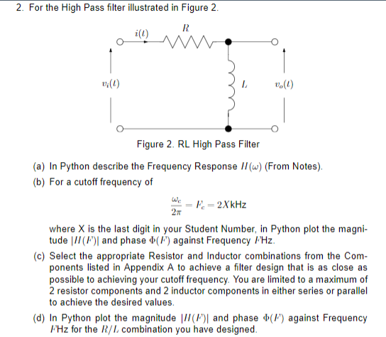
2. For the High Pass filter illustrated in Figure 2. R i(l) v (1) Vo(l) Figure 2. RL High Pass Filter (a) In Python describe the Frequency Response H(w) (From Notes). (b) For a cutoff frequency of F-2XkHz 2TT where X is the last digit in your Student Number, in Python plot the magni- tude // (/) and phase () against Frequency /Hz. (c) Select the appropriate Resistor and Inductor combinations from the Com- ponents listed in Appendix A to achieve a filter design that is as close as possible to achieving your cutoff frequency. You are limited to a maximum of 2 resistor components and 2 inductor components in either series or parallel to achieve the desired values. (d) In Python plot the magnitude (P) and phase (F) against Frequency FHz for the R/L combination you have designed.