The debate over the viability of the program centered on estimated break-even sales - the number...

Transcribed Image Text:

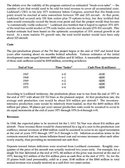
The debate over the viability of the program centered on estimated "break-even sales" - the number of jets that would need to be sold for total revenue to cover all accumulated costs. Lockheed's CEO, in his July 1971 testimony before Congress, asserted that this break-even point would be reached at sales somewhere between 195 and 205 aircraft. At that point, Lockheed had secured only 103 firm orders plus 75 options-to-buy, but they testified that sales would eventually exceed the break-even point and that the project would thus become "a commercially viable endeavor." Lockheed also testified that it hoped to capture 35%-40% of the total free-world market of 775 wide bodies over the next decade (270-310 aircraft). This market estimate had been based on the optimistic assumption of 10% annual growth in air travel. At a more realistic 5 % growth rate, the total world market would have been only about 323 aircraft. Costs The pre-production phases of the Tri Star project began at the end of 1967 and lasted four years after running about six months behind schedule. Various estimates of the initial development costs ranged between $800 million and $1 billion. A reasonable approximation of these cash outflows would be $900 million, occurring as follows: Time "Index" Cash Flow (5 millions) End of Year 1967 1968 1969 1970 1971 1-2 1-3 1-4 -$100 -$200 -$200 -$200 -$200 According to Lockheed testimony, the production phase was to run from the end of 1971 to the end of 1977 with about 210 Tri Stars as the planned output. At that production rate, the average unit production cost would be about $14 million per aircraft.2 The inventory- intensive production costs would be relatively front-loaded, so that the $490 million ($14 million per plane, 35 planes per year) annual production costs could be assumed to occur in six equal increments at the end of years 1971 through 1976 (t-4 through t-9). Revenues In 1968, the expected price to be received for the L-1011 Tri Star was about $16 million per aircraft. These revenue flows would be characterized by a lag of a year to the production cost outflows; annual revenues of $560 million could be assumed to occur in six equal increments at the end of years 1972 through 1977 (t-5 through t-10). Inflation-escalation terms in the contracts ensured that any future inflation-based cost and revenue increases offset each other nearly exactly, thus providing no incremental net cash flow. Deposits toward future deliveries were received from Lockheed customers. Roughly one- quarter of the price of the aircraft was actually received two years early. For example, for a single Tri Star delivered at the end of 1972, $4 million of the price was received at the end of 1970, leaving $12 million of the $16 million price as cash flow at the end of 1972. So, for the 35 planes built (and presumably, sold) in a year, $140 million of the $560 million in total annual revenue was actually received as a cash flow two years earlier. Valuing Capital Investment Projects 298-092 Discount Rate Experts estimated that the cost of capital applicable to Lockheed's cash flows (prior to Tri Star) was in the 9%-10% range. Since the Tri Star project was quite a bit riskier (by any measure) than the typical Lockheed operation, the appropriate discount rate was almost certainly higher than that. Thus, 10% was a reasonable (although possibly generous) estimate of the appropriate discount rate to apply to the Tri Star program's cash flows. Break-Even Revisited In an August 1972 Time magazine article, Lockheed (after receiving government loan guarantees) revised its break-even sales volume: "[Lockheed] claims that it can get back its development costs [about $960 million] and start making a profit by selling 275 Tri Stars."3 Industry analysts had predicted this (actually, they had estimated 300 units to be the break- even volume) even prior to the Congressional hearings. Based on a "learning curve" effect, production costs at these levels (up to 300 units) would average only about $12.5 million per unit, instead of $14 million as above. Had Lockheed been able to produce and sell as many as 500 aircraft, this average cost figure might even have been as low as $11 million per aircraft. A. B. C. D. At originally planned production levels (210 units), what would have been the estimated value of the Tri Star program as of the end of 1967? At "break-even" production of roughly 300 units, did Lockheed break even in terms of net present value? At what sales volume would the Tri Star program have reached true economic (as opposed to accounting) break-even? Was the decision to pursue the Tri Star program a reasonable one? What effects would you predict the adoption of the Tri Star program would have on shareholder value? 3 Time (August 21, 1972), 62. 4 Mitchell Gordon, "Hitched to the Tri Star-Disaster at Lockheed Would Cut a Wide Swathe," Barron's (March 15, 1971), 5-14. 5 In 1971, the American aerospace company, Lockheed, found itself in Congressional hearings seeking a $250 million federal guarantee to secure bank credit required for the completion of the L-1011 Tri Star program. The L-1011 Tri Star Airbus was a wide-bodied commercial jet aircraft with a capacity of up to 400 passengers, competing with the DC-10 triject and the A- 300B airbus. Spokesmen for Lockheed claimed that the Tri Star program was economically sound and that their problem was merely a liquidity crisis caused by some unrelated military contracts. Opposing the guarantee, other parties argued that the Tri Star program had been economically unsound and doomed to financial failure from the very beginning. 1 Facts and situations concerning the Lockheed Tri Star program are taken from U. E. Reinhardt, "Break-Even Analysis for Lockheed's Tri Star: An Application of Financial Theory," Journal of Finance 27 (1972), 821-838, and from House and Senate testimony. The debate over the viability of the program centered on estimated "break-even sales" - the number of jets that would need to be sold for total revenue to cover all accumulated costs. Lockheed's CEO, in his July 1971 testimony before Congress, asserted that this break-even point would be reached at sales somewhere between 195 and 205 aircraft. At that point, Lockheed had secured only 103 firm orders plus 75 options-to-buy, but they testified that sales would eventually exceed the break-even point and that the project would thus become "a commercially viable endeavor." Lockheed also testified that it hoped to capture 35%-40% of the total free-world market of 775 wide bodies over the next decade (270-310 aircraft). This market estimate had been based on the optimistic assumption of 10% annual growth in air travel. At a more realistic 5 % growth rate, the total world market would have been only about 323 aircraft. Costs The pre-production phases of the Tri Star project began at the end of 1967 and lasted four years after running about six months behind schedule. Various estimates of the initial development costs ranged between $800 million and $1 billion. A reasonable approximation of these cash outflows would be $900 million, occurring as follows: Time "Index" Cash Flow (5 millions) End of Year 1967 1968 1969 1970 1971 1-2 1-3 1-4 -$100 -$200 -$200 -$200 -$200 According to Lockheed testimony, the production phase was to run from the end of 1971 to the end of 1977 with about 210 Tri Stars as the planned output. At that production rate, the average unit production cost would be about $14 million per aircraft.2 The inventory- intensive production costs would be relatively front-loaded, so that the $490 million ($14 million per plane, 35 planes per year) annual production costs could be assumed to occur in six equal increments at the end of years 1971 through 1976 (t-4 through t-9). Revenues In 1968, the expected price to be received for the L-1011 Tri Star was about $16 million per aircraft. These revenue flows would be characterized by a lag of a year to the production cost outflows; annual revenues of $560 million could be assumed to occur in six equal increments at the end of years 1972 through 1977 (t-5 through t-10). Inflation-escalation terms in the contracts ensured that any future inflation-based cost and revenue increases offset each other nearly exactly, thus providing no incremental net cash flow. Deposits toward future deliveries were received from Lockheed customers. Roughly one- quarter of the price of the aircraft was actually received two years early. For example, for a single Tri Star delivered at the end of 1972, $4 million of the price was received at the end of 1970, leaving $12 million of the $16 million price as cash flow at the end of 1972. So, for the 35 planes built (and presumably, sold) in a year, $140 million of the $560 million in total annual revenue was actually received as a cash flow two years earlier. Valuing Capital Investment Projects 298-092 Discount Rate Experts estimated that the cost of capital applicable to Lockheed's cash flows (prior to Tri Star) was in the 9%-10% range. Since the Tri Star project was quite a bit riskier (by any measure) than the typical Lockheed operation, the appropriate discount rate was almost certainly higher than that. Thus, 10% was a reasonable (although possibly generous) estimate of the appropriate discount rate to apply to the Tri Star program's cash flows. Break-Even Revisited In an August 1972 Time magazine article, Lockheed (after receiving government loan guarantees) revised its break-even sales volume: "[Lockheed] claims that it can get back its development costs [about $960 million] and start making a profit by selling 275 Tri Stars."3 Industry analysts had predicted this (actually, they had estimated 300 units to be the break- even volume) even prior to the Congressional hearings. Based on a "learning curve" effect, production costs at these levels (up to 300 units) would average only about $12.5 million per unit, instead of $14 million as above. Had Lockheed been able to produce and sell as many as 500 aircraft, this average cost figure might even have been as low as $11 million per aircraft. A. B. C. D. At originally planned production levels (210 units), what would have been the estimated value of the Tri Star program as of the end of 1967? At "break-even" production of roughly 300 units, did Lockheed break even in terms of net present value? At what sales volume would the Tri Star program have reached true economic (as opposed to accounting) break-even? Was the decision to pursue the Tri Star program a reasonable one? What effects would you predict the adoption of the Tri Star program would have on shareholder value? 3 Time (August 21, 1972), 62. 4 Mitchell Gordon, "Hitched to the Tri Star-Disaster at Lockheed Would Cut a Wide Swathe," Barron's (March 15, 1971), 5-14. 5 In 1971, the American aerospace company, Lockheed, found itself in Congressional hearings seeking a $250 million federal guarantee to secure bank credit required for the completion of the L-1011 Tri Star program. The L-1011 Tri Star Airbus was a wide-bodied commercial jet aircraft with a capacity of up to 400 passengers, competing with the DC-10 triject and the A- 300B airbus. Spokesmen for Lockheed claimed that the Tri Star program was economically sound and that their problem was merely a liquidity crisis caused by some unrelated military contracts. Opposing the guarantee, other parties argued that the Tri Star program had been economically unsound and doomed to financial failure from the very beginning. 1 Facts and situations concerning the Lockheed Tri Star program are taken from U. E. Reinhardt, "Break-Even Analysis for Lockheed's Tri Star: An Application of Financial Theory," Journal of Finance 27 (1972), 821-838, and from House and Senate testimony.