The excel data is in this link: https://drive.google.com/open?id=1fBMESYbIdFm31llrb26p_nCMHTcrTeCV

I did wrong in the table to get the correct answer but the formula seems to be right

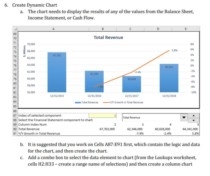
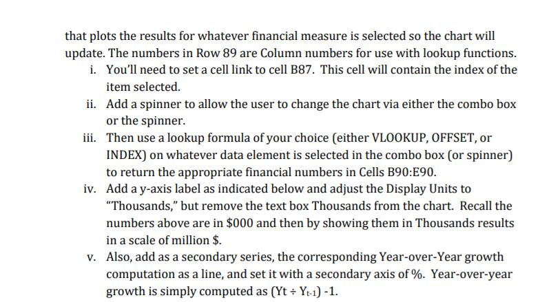
6. Create Dynamic Chart The chart needs to display the results of any of the values from the Balance Sheet, Income Statement, or Cash Flow a. Total Revenue 70 71 72 73 70,000 68,000 66,000 64,000 62,000 60,000 58,000 56,000 67,702 75 76 64,341 -2.4% 78 79 80 50,828 82 83 84 85 86 87 Index of selected component 88 Select the Financial Statement component to chart: 89 Column Index Num 90 Total Revenue 91 Y/Y Growth in Total Revenue 12/31/2016 12/31/2017 12/31/2018 Total RevenueY/N Growth in Total Revenue Total Revenue 67,702,000 62,346,000 60,828,000 2.4% 64,341,000 b. It is suggested that you work on Cells A87:E91 first, which contain the logic and data for the chart, and then create the chart. Add a combo box to select the data element to chart (from the Lookups worksheet, cells H2:H33- create a range name of selections) and then create a column chart c. that plots the results for whatever financial measure is selected so the chart will update. The numbers in Row 89 are Column numbers for use with lookup functions. i. You'll need to set a cell link to cell B87. This cell will contain the index of the item selected. Add a spinner to allow the user to change the chart via either the combo box or the spinner. Then use a lookup formula of your choice (either VLOOKUP, OFFSET, or INDEX) on whatever data element is selected in the combo box (or spinner) to return the appropriate financial numbers in Cells B90:E90. Add a y-axis label as indicated below and adjust the Display Units to "Thousands," but remove the text box Thousands from the chart. Recall the numbers above are in $000 and then by showing them in Thousands results in a scale of million $. Also, add as a secondary series, the corresponding Year-over-Year growth computation as a line, and set it with a secondary axis of%. Year-over-year growth is simply computed as (Yt Y1-1 ii. iii. iv. v. 6. Create Dynamic Chart The chart needs to display the results of any of the values from the Balance Sheet, Income Statement, or Cash Flow a. Total Revenue 70 71 72 73 70,000 68,000 66,000 64,000 62,000 60,000 58,000 56,000 67,702 75 76 64,341 -2.4% 78 79 80 50,828 82 83 84 85 86 87 Index of selected component 88 Select the Financial Statement component to chart: 89 Column Index Num 90 Total Revenue 91 Y/Y Growth in Total Revenue 12/31/2016 12/31/2017 12/31/2018 Total RevenueY/N Growth in Total Revenue Total Revenue 67,702,000 62,346,000 60,828,000 2.4% 64,341,000 b. It is suggested that you work on Cells A87:E91 first, which contain the logic and data for the chart, and then create the chart. Add a combo box to select the data element to chart (from the Lookups worksheet, cells H2:H33- create a range name of selections) and then create a column chart c. that plots the results for whatever financial measure is selected so the chart will update. The numbers in Row 89 are Column numbers for use with lookup functions. i. You'll need to set a cell link to cell B87. This cell will contain the index of the item selected. Add a spinner to allow the user to change the chart via either the combo box or the spinner. Then use a lookup formula of your choice (either VLOOKUP, OFFSET, or INDEX) on whatever data element is selected in the combo box (or spinner) to return the appropriate financial numbers in Cells B90:E90. Add a y-axis label as indicated below and adjust the Display Units to "Thousands," but remove the text box Thousands from the chart. Recall the numbers above are in $000 and then by showing them in Thousands results in a scale of million $. Also, add as a secondary series, the corresponding Year-over-Year growth computation as a line, and set it with a secondary axis of%. Year-over-year growth is simply computed as (Yt Y1-1 ii. iii. iv. v