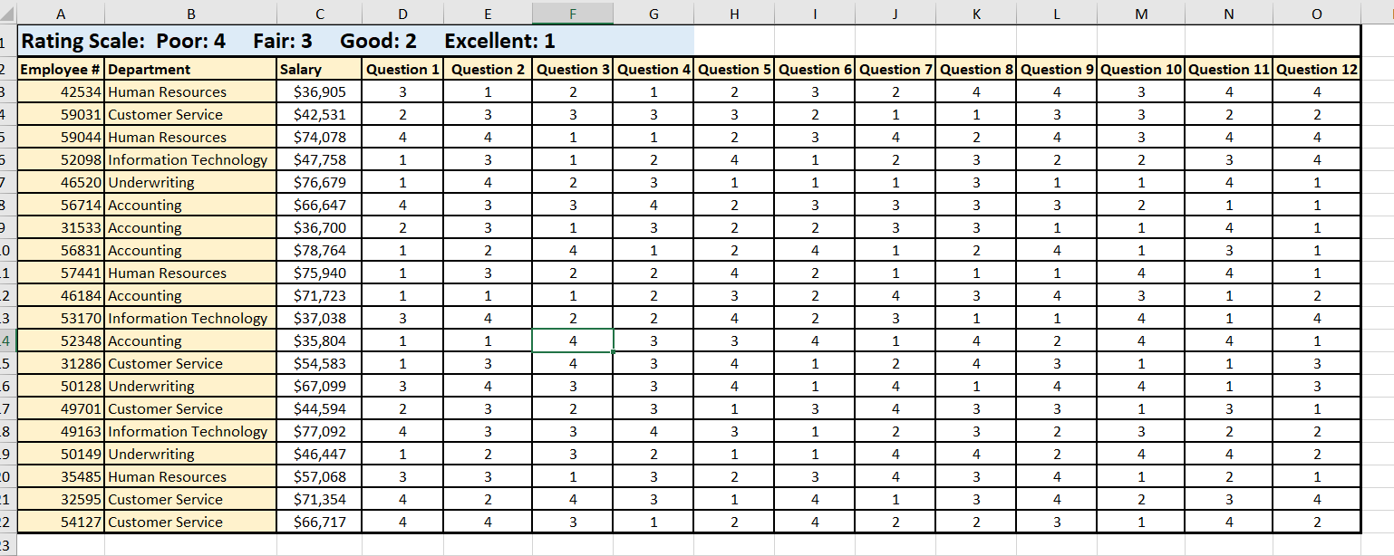
The first sheet is individual responses, and second sheet is Average Q$3$ Rating by Department sheet. Third sheet is for problem $3.$ Write a formula in cell $$Average Q$3$ Rating by Department$!$B$3,$ which can be copied to cell

$$Average Q$3$ Rating by Department$!$B$7,$ to calculate the average rating by department for

question $3.($Round the number to the nearest $10$th$.)$

We will break down this function in steps.

$$ Because there is only one criteria, use the AVERAGEIF function and add the $ to each column and row reference where

it is necessary. Copy the formula down. Check your answers to make sure the function works properly.

$$ Select cell $$Average Q$3$ Rating by Department$!$B$3$ and add the round function to the formula. Check your answers to

make sure the function works properly.

When using the AVERAGEIF function, if there are no cells that meet the criteria, Excel will display a #DIV$/0!$ error. You

want the cell to display as $0$ or as dashes if the sheet is in Accounting format, so to avoid the #DIV$/0!$ error, you can use

the IFERROR function.

Syntax of complete function: IFERROR$($ROUND$($AVERAGEIF$(.........),...),...)\backslash$table$[[,,$Ques $1,$Ques $2,$Ques $3,$Ques $4,$Ques $5,$Ques $6,$Ques $7,$Ques $8,$Ques $9,$Ques $10,$Ques $11,$Ques $12],[$Response$,,\backslash$table$[[$Availability$],[$of a clear$],[$description$]],\backslash$table$[[$Feedback$],[$about job$],[$performance$]],\backslash$table$[[$Sufficient$],[$training$],[$opportunities$]],\backslash$table$[[$Availability of$],[$follow$-$up$],[$training$]],\backslash$table$[[$Availability of a$],[$supervisor to$],[$answer your$],[$questions$]],\backslash$table$[[$Feedback and$],[$evaluation$],[$regarding your$],[$performance$]],\backslash$table$[[$Recognition by$],[$your supervisor$],[$for your$],[$accomolishments$]],\backslash$table$[[$Fariness in$],[$supervision$],[$and$],[$employment$],[$opportunities$]],\backslash$table$[[$Relationship$],[$with your$],[$supervisor$]],\backslash$table$[[$Your rate$],[$of pay for$],[$your work$]],\backslash$table$[[$Paid time$],[$off you$],[$receive$]],\backslash$table$[[$Benefits$],[$you$],[$receive$]]],[$oor$,4,5,5,4,2,5,4,6,4,7,5,8,5],[$air$,3,4,9,6,9,4,5,3,9,5,5,4,2],[$iood$,2,3,3,5,5,7,5,5,3,4,3,3,5],[$xcellent$,1,8,3,5,4,4,6,6,4,4,7,5,8]]$