The model below is a 2 stages least squares regression model using 4 insturments

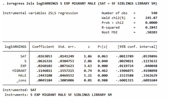
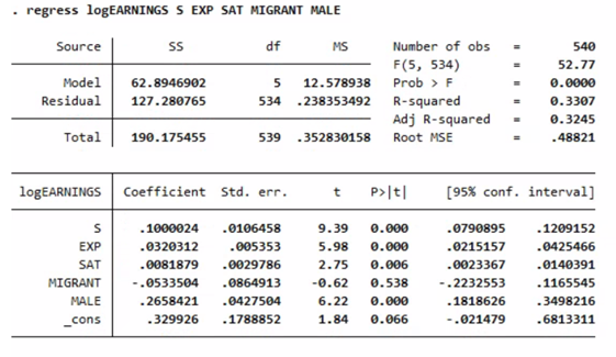
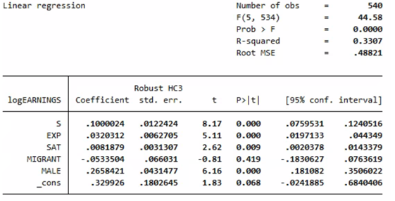
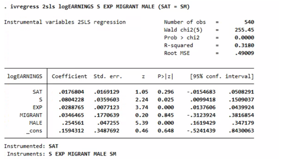
Compare the results of this model with the 3 models below, an OLS regression, an OLS with heteroskedasticty-robust standard errors and an 2sls regression using 1 insutrument respectively.

. ivregress 2sls logEARNINGS S EXP MIGRANT MALE (SAT = SE SIBLINGS LIBRARY SM) Instrumental variables 25Ls regression Number of obs Wald chi2(5) Prob > chi2 0.0000 R-squared 0.2843 Root MSE 540 245.87 .50203 logEARNINGS Coefficient Std. err. P>z! [95% conf. interval] SAT s EXP MIGRANT MALE _cons .0263053 .0626326 .0260102 . 1146011 .2443108 .0045184 .0141249 .0304753 .0071623 . 1557215 .0469152 .3085006 1.86 2.06 3.63 0.74 5.21 @.01 0.063 0.040 0.000 0.462 0.000 0.988 -.0013789 .0029021 .0119724 -.1906075 . 1523588 -.6001315 .0539896 .1223632 .040048 .4198098 .3362629 .6091684 Instrumented: SAT Instruments: S EXP MIGRANT MALE SE SIBLINGS LIBRARY SM regress logEARNINGS S EXP SAT MIGRANT MALE Source SS df MS Model Residual 62.8946902 127.280765 5 534 12.578938 .238353492 Number of obs F(5, 534) Prob > F R-squared Adj R-squared Root MSE 540 52.77 0.0000 0.3307 0.3245 .48821 Total 190.175455 539 .352830158 = logEARNINGS coefficient Std. err. t P>It [95% conf. interval) s EXP SAT MIGRANT MALE _cons .1000024 .0320312 .0081879 -.0533504 .2658421 .329926 .0106458 .005353 .0029786 .0864913 .0427504 .1788852 9.39 5.98 2.75 -0.62 6.22 1.84 0.000 0.000 0.006 .538 0.000 0.066 .0790895 .0215157 0023367 - .2232553 .1818626 -.021479 .1209152 .0425466 .0140391 1165545 .3498216 .6813311 Linear regression 540 Number of obs F(5, 534) Prob > F R-squared Root MSE 44.58 0.0000 0.3307 .48821 Robust HC3 logEARNINGS Coefficient std. err. t P>It! [95% conf. interval] S EXP SAT MIGRANT MALE .1000024 .0320312 .0081879 -.0533504 .2658421 . 329926 .0122424 .0062705 .0031307 .066031 .0431477 .1802645 8.17 5.11 2.62 -0.81 6.16 1.83 0.000 0.000 0.009 0.419 0.000 0.068 .0759531 .0197133 .0020378 -.1830627 . 181082 -.0241885 . 1240516 .044349 .0143379 .0763619 .3506022 .6840406 cons . ivregress 2sls logEARNINGS S EXP MIGRANT MALE (SAT = SM) Instrumental variables 25LS regression Number of obs Wald chi2(5) Prob > chi2 R-squared Root MSE 540 255.45 0.0000 0.3180 .49009 logEARNINGS Coefficient Std. err . P>21 [95% conf. interval] SAT S EXP MIGRANT MALE _cons .0176804 .0804228 .0288765 .0346465 .254561 . 1594312 .0169129 .0359603 .0077123 . 1770639 .047255 .3487692 1.05 2.24 3.74 .20 5.39 0.46 0.296 0.025 0.000 0.845 0.000 0.648 -.0154683 .0099418 .0137606 . 3123924 . 1619429 -.5241439 .0508291 . 1509037 .0439924 3816854 . 347179 .8430063 Instrumented: SAT Instruments: S EXP MIGRANT MALE SM . ivregress 2sls logEARNINGS S EXP MIGRANT MALE (SAT = SE SIBLINGS LIBRARY SM) Instrumental variables 25Ls regression Number of obs Wald chi2(5) Prob > chi2 0.0000 R-squared 0.2843 Root MSE 540 245.87 .50203 logEARNINGS Coefficient Std. err. P>z! [95% conf. interval] SAT s EXP MIGRANT MALE _cons .0263053 .0626326 .0260102 . 1146011 .2443108 .0045184 .0141249 .0304753 .0071623 . 1557215 .0469152 .3085006 1.86 2.06 3.63 0.74 5.21 @.01 0.063 0.040 0.000 0.462 0.000 0.988 -.0013789 .0029021 .0119724 -.1906075 . 1523588 -.6001315 .0539896 .1223632 .040048 .4198098 .3362629 .6091684 Instrumented: SAT Instruments: S EXP MIGRANT MALE SE SIBLINGS LIBRARY SM regress logEARNINGS S EXP SAT MIGRANT MALE Source SS df MS Model Residual 62.8946902 127.280765 5 534 12.578938 .238353492 Number of obs F(5, 534) Prob > F R-squared Adj R-squared Root MSE 540 52.77 0.0000 0.3307 0.3245 .48821 Total 190.175455 539 .352830158 = logEARNINGS coefficient Std. err. t P>It [95% conf. interval) s EXP SAT MIGRANT MALE _cons .1000024 .0320312 .0081879 -.0533504 .2658421 .329926 .0106458 .005353 .0029786 .0864913 .0427504 .1788852 9.39 5.98 2.75 -0.62 6.22 1.84 0.000 0.000 0.006 .538 0.000 0.066 .0790895 .0215157 0023367 - .2232553 .1818626 -.021479 .1209152 .0425466 .0140391 1165545 .3498216 .6813311 Linear regression 540 Number of obs F(5, 534) Prob > F R-squared Root MSE 44.58 0.0000 0.3307 .48821 Robust HC3 logEARNINGS Coefficient std. err. t P>It! [95% conf. interval] S EXP SAT MIGRANT MALE .1000024 .0320312 .0081879 -.0533504 .2658421 . 329926 .0122424 .0062705 .0031307 .066031 .0431477 .1802645 8.17 5.11 2.62 -0.81 6.16 1.83 0.000 0.000 0.009 0.419 0.000 0.068 .0759531 .0197133 .0020378 -.1830627 . 181082 -.0241885 . 1240516 .044349 .0143379 .0763619 .3506022 .6840406 cons . ivregress 2sls logEARNINGS S EXP MIGRANT MALE (SAT = SM) Instrumental variables 25LS regression Number of obs Wald chi2(5) Prob > chi2 R-squared Root MSE 540 255.45 0.0000 0.3180 .49009 logEARNINGS Coefficient Std. err . P>21 [95% conf. interval] SAT S EXP MIGRANT MALE _cons .0176804 .0804228 .0288765 .0346465 .254561 . 1594312 .0169129 .0359603 .0077123 . 1770639 .047255 .3487692 1.05 2.24 3.74 .20 5.39 0.46 0.296 0.025 0.000 0.845 0.000 0.648 -.0154683 .0099418 .0137606 . 3123924 . 1619429 -.5241439 .0508291 . 1509037 .0439924 3816854 . 347179 .8430063 Instrumented: SAT Instruments: S EXP MIGRANT MALE SM