The question is about Optimization or Numerical linear algebra with MATLAB.

Maybe you can write the MATLAB code.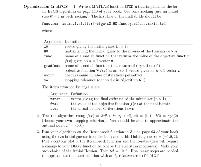

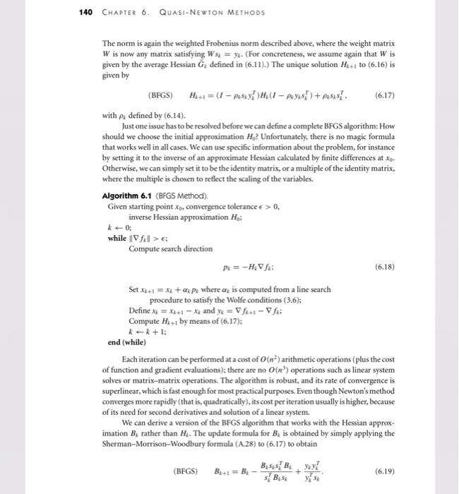
Optimization 1: BFGS 1. Write a MATLAB function BFGS.m that implements the ba sic BFGS algorithm on page 140 of your book. Use backtracking (use an initial step1 in backtracking). The first line of the matlab file should be function [xstar , fval ,iter]=bfgs (x0,Ho,func , gradfunc,maxit ,tol) wher Argument Definition vector giving the initial guess (n 1) matrix giving the initial guess to the inverse of the Hessian (n n) name of a matlab function that returns the value of the objective function f(x) given an n 1 vector x HO func gradfunc name of a matlab function that returns the gradient of the maxit tol objective function f(x) as an n 1 vector given an n 1 vector x the maximum number of iterations permitted stopping tolerance (denoted e in Algorithm 6.1) The items returned by bfgs.m are Argument Definition xstar fvalthe value of the objective function f() at the final iterate iter vector giving the final estimate of the minimizer (n 1 the actual number of iterations taken 2. Test the algorithm using f(x)-3rf + 2x1x2 +:0-[1:1), H0 = eye(2) (choose your own stopping criterion). You should be able to approximate the optimal point x* = (0,0) 3. Run your algorithm on the Rosenbrock function in 3.1 on page 63 of your book using the two initial guesses from the book and a third initial guess 0 = ( 1.9.2) Plot a contour plot of the Rosenbrock function and the iterates (this will require a change to your BFGS function to plot as the algorithm progresses). Make your own choice of the initial Hessian. Take tol = 10-4. How many steps are needed to approximate the exact solution with an 12 relative error of 0.01%? Optimization 1: BFGS 1. Write a MATLAB function BFGS.m that implements the ba sic BFGS algorithm on page 140 of your book. Use backtracking (use an initial step1 in backtracking). The first line of the matlab file should be function [xstar , fval ,iter]=bfgs (x0,Ho,func , gradfunc,maxit ,tol) wher Argument Definition vector giving the initial guess (n 1) matrix giving the initial guess to the inverse of the Hessian (n n) name of a matlab function that returns the value of the objective function f(x) given an n 1 vector x HO func gradfunc name of a matlab function that returns the gradient of the maxit tol objective function f(x) as an n 1 vector given an n 1 vector x the maximum number of iterations permitted stopping tolerance (denoted e in Algorithm 6.1) The items returned by bfgs.m are Argument Definition xstar fvalthe value of the objective function f() at the final iterate iter vector giving the final estimate of the minimizer (n 1 the actual number of iterations taken 2. Test the algorithm using f(x)-3rf + 2x1x2 +:0-[1:1), H0 = eye(2) (choose your own stopping criterion). You should be able to approximate the optimal point x* = (0,0) 3. Run your algorithm on the Rosenbrock function in 3.1 on page 63 of your book using the two initial guesses from the book and a third initial guess 0 = ( 1.9.2) Plot a contour plot of the Rosenbrock function and the iterates (this will require a change to your BFGS function to plot as the algorithm progresses). Make your own choice of the initial Hessian. Take tol = 10-4. How many steps are needed to approximate the exact solution with an 12 relative error of 0.01%