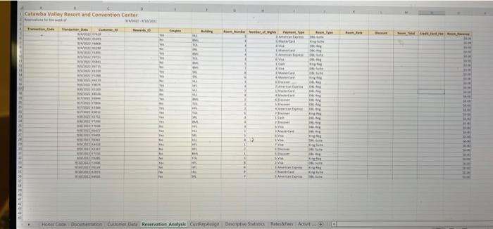
The Reservation_Analysis sheet displays data regarding reservations made by customers during the week of September 4, 2022 through September 10, 2022. You must help the manager of CVRCC complete the Reservation_Analysis sheet. Enter an XLOOKUP function in cell D5 of the Reservation_Analysis sheet. The lookup function must find the Customer_ID (cell C5) in the Customer_Data sheet and return the Rewards_ID. (Note: N/A is displayed if the customer is not a rewards member.) If the Customer_ID is not found in the Customer_Data sheet, the following text should be displayed: Not Found. (Do not include the period.) Copy the formula in cell D5 down the column to cell D36. Create a Transaction_Code for each of the transactions on the Reservation_Analysis sheet. Place a formula in cell A5 of the Reservation_Analysis sheet that uses the TEXT, RIGHT, IF and LEFT functions to create a transaction code. The transaction code should begin with the transaction date in YYMMDD format. The date should be followed by a dash (). The dash should be followed by the last 4 characters of the Customer_ID. The last four characters of the Customer_ID should be followed by the first 2 characters of the Rewards.ID if the customer is a rewards member. If the customer is not a rewards member, the letters XX should be used instead of the first 2 characters of the Rewards ID. After the first 2 characters of the Rewards_ID or the XX, there should be a dash (-). The dash should be followed by the Building code and the Room_Number. For example, a Transaction_Code for a reservation with a Transaction_Date of 9/5/2022, a Customer_ID of X1234, a Rewards_ID of 9876Y, Building of SRL and Room_Number of 2 would look like this: 220905-123498-SRL2. Copy the formula in cell A5 to cell range A6:A36. Go to the Rates\&Fees sheet and name the following ranges. Cell range A17:B20 should be named BML. Cell range A24:B27 should be named HFL. Cell range A31:B34 should be named HLL. Cell range A38:B41 should be named SRL and cell range A45:B48 should be named TOL. Enter a formula in cell K5 of the Reservation_Analysis sheet that displays the correct room rate. Use a VLOOKUP function and an INDIRECT function to do this. The room rate depends on both the Building and the Room_Type. (Room rates are listed on the Rates\&Fees sheet.) Copy the formula in cell K5 down the column to K 36 . Hint: Room rates for each different building listed on the Rates\&Fees sheet have been named. The Reservation_Analysis sheet displays data regarding reservations made by customers during the week of September 4, 2022 through September 10, 2022. You must help the manager of CVRCC complete the Reservation_Analysis sheet. Enter an XLOOKUP function in cell D5 of the Reservation_Analysis sheet. The lookup function must find the Customer_ID (cell C5) in the Customer_Data sheet and return the Rewards_ID. (Note: N/A is displayed if the customer is not a rewards member.) If the Customer_ID is not found in the Customer_Data sheet, the following text should be displayed: Not Found. (Do not include the period.) Copy the formula in cell D5 down the column to cell D36. Create a Transaction_Code for each of the transactions on the Reservation_Analysis sheet. Place a formula in cell A5 of the Reservation_Analysis sheet that uses the TEXT, RIGHT, IF and LEFT functions to create a transaction code. The transaction code should begin with the transaction date in YYMMDD format. The date should be followed by a dash (). The dash should be followed by the last 4 characters of the Customer_ID. The last four characters of the Customer_ID should be followed by the first 2 characters of the Rewards.ID if the customer is a rewards member. If the customer is not a rewards member, the letters XX should be used instead of the first 2 characters of the Rewards ID. After the first 2 characters of the Rewards_ID or the XX, there should be a dash (-). The dash should be followed by the Building code and the Room_Number. For example, a Transaction_Code for a reservation with a Transaction_Date of 9/5/2022, a Customer_ID of X1234, a Rewards_ID of 9876Y, Building of SRL and Room_Number of 2 would look like this: 220905-123498-SRL2. Copy the formula in cell A5 to cell range A6:A36. Go to the Rates\&Fees sheet and name the following ranges. Cell range A17:B20 should be named BML. Cell range A24:B27 should be named HFL. Cell range A31:B34 should be named HLL. Cell range A38:B41 should be named SRL and cell range A45:B48 should be named TOL. Enter a formula in cell K5 of the Reservation_Analysis sheet that displays the correct room rate. Use a VLOOKUP function and an INDIRECT function to do this. The room rate depends on both the Building and the Room_Type. (Room rates are listed on the Rates\&Fees sheet.) Copy the formula in cell K5 down the column to K 36 . Hint: Room rates for each different building listed on the Rates\&Fees sheet have been named