

Question: The sales data for two years are as follows. Data are aggregated with two months of sales in each period. table [ [ MoNTHS
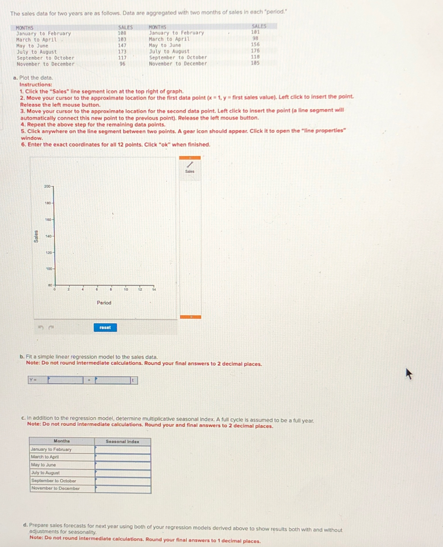
The sales data for two years are as follows. Data are aggregated with two months of sales in each "period."
tableMoNTHSSALES,,MoNTHS,SALESJanuary to February,January to February,March to April,March to April,May to June,May to June,July to August,July to August,Septenber to October,September to October,Novenber to Decenber,Novenber to Decenber,
a Plot the data.
Instructions:
Click the "Sales" line segment icon at the top right of graph.
Move your cursor to the approximate location for the first data point first sales value Left click to insert the point. Release the left mouse button.
Move your cursor to the approximate location for the second data point. Left click to insert the point fa line segment will automatically connect this new point to the previous point Release the left mouse button.
Repeat the above step for the remaining data points.
Click anywhere on the line segment between two points. A gear icon should appear. Click it to open the "line properties" window.
Enter the exact coordinates for all points. Click ok when finished.
b Fit a simple linear regression model to the sales data.
Note: Do not round intermediate calculations. Round your final answers to decimal places.
c In addition to the regression model, determine multiplicative seasonal index. A full cycle is assumed to be a full year, Note: Do not round intermediate calculations. Round your and final answers to decimal places.
tableMonthsSeasonal IndexJanuary to February,March to April,May to June,July to August,September to October,November to December,
d Prepare
b Fit a simple linear regression model to the sales data.
Note: Do not round intermediate calculations. Round your final answers to decimal places.
c In addition to the regression model, determine multiplicative seasonal index. A full cycle is assumed to be a full year. Note: Do not round intermediate calculations. Round your and final answers to decimal places.
tableMonthsSeasonal Index.January to February,March to April,May to June,July to Augusi,September to October,November to December,
d Prepare sales forecasts for next year using both of your regression models derived above to show results both with and without adjustments for seasonality.
Note: Do not round intermediate calculations, Round your final answers to decimal places.
tableMonthsForecastJanuary to February,March to April,May to June,July to August,September to October,November to December,
The sales data for two years are as follows. Data are aggregated with two months of sales in each "period."
tableMoNTHSSALES,NoNTHS,SAtESJanuary to February,January to February,March to April,March to April,May to June,May to June,July to August,July to August,September to October,September to October,Novenber to December,November to Decenber,
a Plot the data.
Instructions:
Click the "Sales" line segment icon at the top right of graph.
Move your cursor to the approximate location for the first data point first sales value Left click to insert the point. Release the left mouse button.
Move your cursor to the approximate location for the second data point. Left click to insert the point a line segment will automatically connect this new point to the previous point Release the left mouse button.
Repeat the above step for the remaining data points.
Click anywhere on the line segment between two points. A gear icon should appear. Click it to open the "line properties" window.
Enter the exact coordinates for all polnts. Click ok when finished.
b Fit a simple linear regression model to the sales data.
Note: Do not round intermediate calculations. Round your final answers to decimal places.
c In addition to the regression model, determine multiplicative seasonal index. A full cycle is assumed to be a full year. Note: Do not round intermediate calculations. Round your and final answers to decimal places.
tableMonthsSeasonal IndoxJanuary to February,March to April,May to June,July to August,Septomber to October,November to Decomber,
d Prepare sales forecasts for next year using both of your regression models derived above to show results both with and without adjustments for seasonality.
Note: Do not round intermediate calculations. Round your final answers to decimal places.
Step by Step Solution
There are 3 Steps involved in it
1 Expert Approved Answer
Step: 1 Unlock

Question Has Been Solved by an Expert!
Get step-by-step solutions from verified subject matter experts
Step: 2 Unlock
Step: 3 Unlock