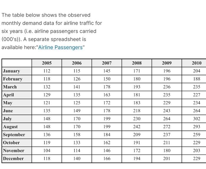
The table below shows the observed monthly demand data for airline traffic for six years (i.e. airline passengers carried (000's)). A separate spreadsheet is available here:"Airline Passengers" 2007 2008 2010 2005 112 2006 115 2009 196 145 171 204 January February March 118 126 150 180 196 188 132 141 178 193 236 235 129 135 163 181 235 227 121 125 172 183 234 229 243 135 149 178 218 April | May June July August September October 264 302 148 170 199 230 264 199 242 272 293 148 136 119 170 158 184 209 237 259 133 211 229 162 146 191 172 November 104 114 180 203 December 118 140 166 194 201 229 In the following questions we will find estimates of the trend and of the seasonal factors. There are many ways to do this; this is not necessarily the only way. We will use this question to illustrate a reasonable and practical way for estimating these factors. We will do this step by step. We first estimate the trend based on the six years (72 months) of observed data. A common way is to use linear regression to determine the best linear model that fits the data. The linear model is specified by a slope term and an intercept term. The slope is the same as the trend, namely the average amount by which demand increases in each month. The intercept is an estimate of the deseasonalized demand at time zero; in this case this corresponds to an estimate of deseasonalized demand in December 2004. In Excel, we find the slope term and the intercept term using the SLOPE and INTERCEPT functions. One can find online many help videos and other material for using these functions. In this case the "y variables" will be the monthly demand that we want to predict; and you should set the corresponding x variables to be the months, numbered from 1 to 72. That is, we use 1 for January 2005, 2 for February 2005, ... and 72 for December 2010. We will use the slope as our estimate of the trend; and we will use the intercept as the estimate of the deseasonalized demand for December 2004. We can now use the estimate of the trend and the estimate of the deseasonalized demand for December 2004 to determine an estimate of the deseasonalized demand for each month. Then our estimate of the deseasonalized demand for month tis given by: S, = S, +txB. This is effectively the linear model from the regression. We are now ready to estimate the seasonal factors: seasonal factors: Compute the estimate of the deseasonalized demand for month tas given above. Divide each monthly demand observation by its corresponding deseasonalized demand estimate to calculate the seasonal factors for each month of observed data. That is, the seasonal factor in month tis d/S, where d, is the demand observation for month t. Average the factors for each month. That is, average all the factors corresponding January, all the factors corresponding to February, and so on. The resulting averages are the 12 seasonal factors, which should add to exactly 12. If they do not add to 12, then we normalize the factors by 12/ multiplying each one by where ci is the estimate for the seasonal factor, before normalization. Determine the forecast for seasonalized demand in the following months, as of December 2010 (Up to two decimal places): January 2011 July 2011 February 2012 October 2012 The table below shows the observed monthly demand data for airline traffic for six years (i.e. airline passengers carried (000's)). A separate spreadsheet is available here:"Airline Passengers" 2007 2008 2010 2005 112 2006 115 2009 196 145 171 204 January February March 118 126 150 180 196 188 132 141 178 193 236 235 129 135 163 181 235 227 121 125 172 183 234 229 243 135 149 178 218 April | May June July August September October 264 302 148 170 199 230 264 199 242 272 293 148 136 119 170 158 184 209 237 259 133 211 229 162 146 191 172 November 104 114 180 203 December 118 140 166 194 201 229 In the following questions we will find estimates of the trend and of the seasonal factors. There are many ways to do this; this is not necessarily the only way. We will use this question to illustrate a reasonable and practical way for estimating these factors. We will do this step by step. We first estimate the trend based on the six years (72 months) of observed data. A common way is to use linear regression to determine the best linear model that fits the data. The linear model is specified by a slope term and an intercept term. The slope is the same as the trend, namely the average amount by which demand increases in each month. The intercept is an estimate of the deseasonalized demand at time zero; in this case this corresponds to an estimate of deseasonalized demand in December 2004. In Excel, we find the slope term and the intercept term using the SLOPE and INTERCEPT functions. One can find online many help videos and other material for using these functions. In this case the "y variables" will be the monthly demand that we want to predict; and you should set the corresponding x variables to be the months, numbered from 1 to 72. That is, we use 1 for January 2005, 2 for February 2005, ... and 72 for December 2010. We will use the slope as our estimate of the trend; and we will use the intercept as the estimate of the deseasonalized demand for December 2004. We can now use the estimate of the trend and the estimate of the deseasonalized demand for December 2004 to determine an estimate of the deseasonalized demand for each month. Then our estimate of the deseasonalized demand for month tis given by: S, = S, +txB. This is effectively the linear model from the regression. We are now ready to estimate the seasonal factors: seasonal factors: Compute the estimate of the deseasonalized demand for month tas given above. Divide each monthly demand observation by its corresponding deseasonalized demand estimate to calculate the seasonal factors for each month of observed data. That is, the seasonal factor in month tis d/S, where d, is the demand observation for month t. Average the factors for each month. That is, average all the factors corresponding January, all the factors corresponding to February, and so on. The resulting averages are the 12 seasonal factors, which should add to exactly 12. If they do not add to 12, then we normalize the factors by 12/ multiplying each one by where ci is the estimate for the seasonal factor, before normalization. Determine the forecast for seasonalized demand in the following months, as of December 2010 (Up to two decimal places): January 2011 July 2011 February 2012 October 2012