The variables included in the worksheet are, for the first question: Real GDP per capita at...

Transcribed Image Text:

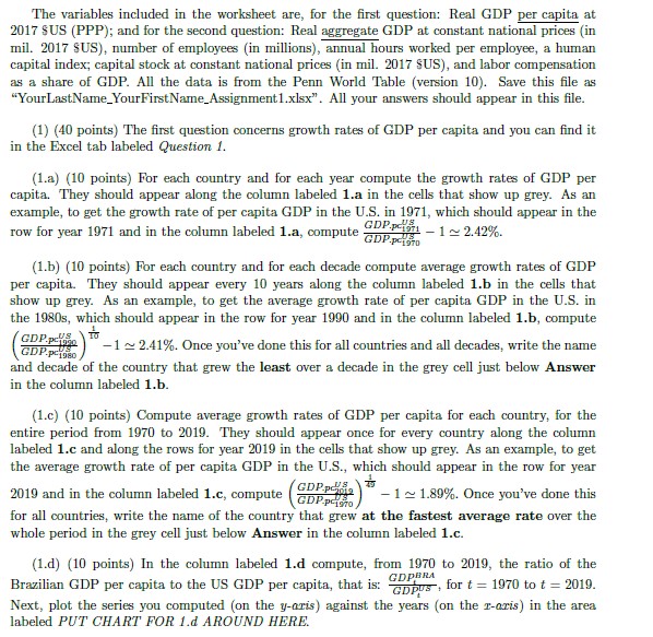
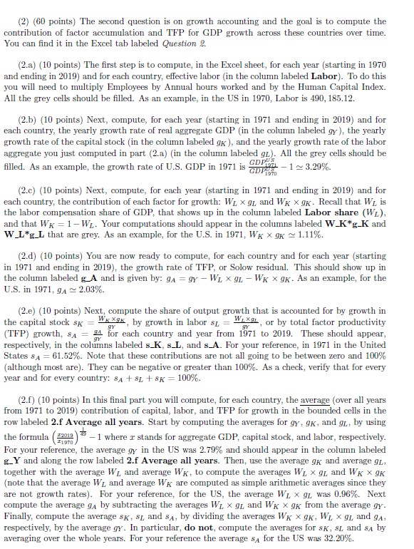
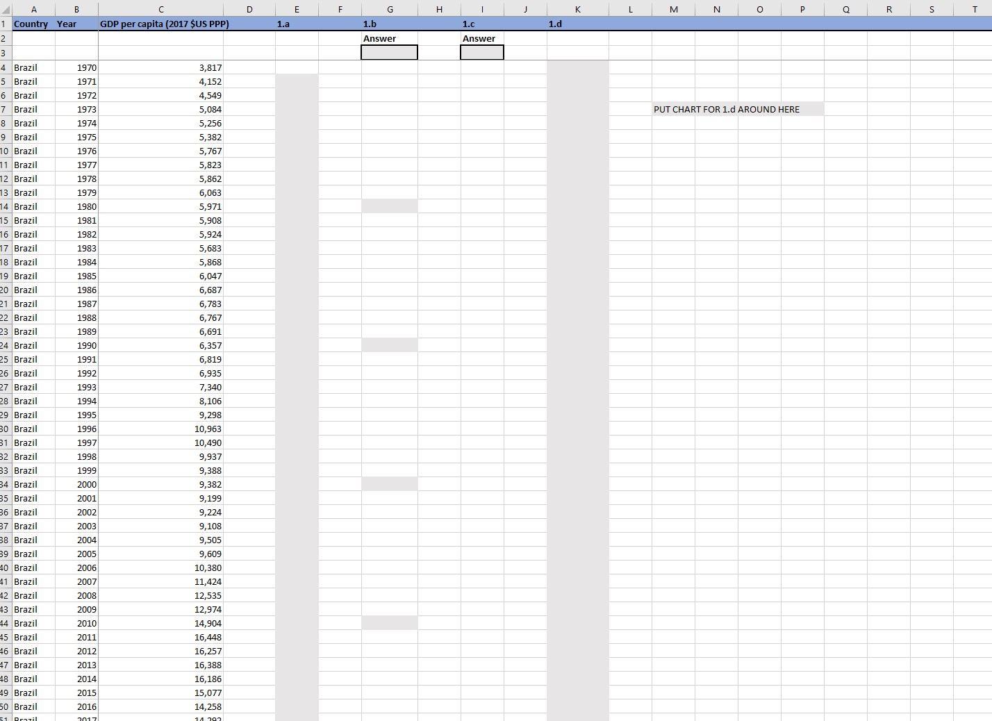
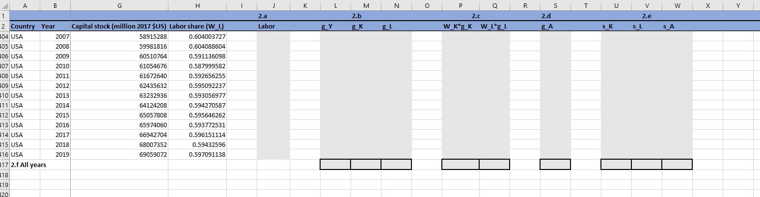
The variables included in the worksheet are, for the first question: Real GDP per capita at 2017 $US (PPP); and for the second question: Real aggregate GDP at constant national prices (in mil. 2017 $US), number of employees (in millions), annual hours worked per employee, a human capital index; capital stock at constant national prices (in mil. 2017 $US), and labor compensation as a share of GDP. All the data is from the Penn World Table (version 10). Save this file as "YourLastName_YourFirst Name Assignment 1.xlsx". All your answers should appear in this file. (1) (40 points) The first question concerns growth rates of GDP per capita and you can find it in the Excel tab labeled Question 1. (1.a) (10 points) For each country and for each year compute the growth rates of GDP per capita. They should appear along the column labeled 1.a in the cells that show up grey. As an example, to get the growth rate of per capita GDP in the U.S. in 1971, which should appear in the row for year 1971 and in the column labeled 1.a, compute GDP-1~2.42%. GDP.1970 (1.b) (10 points) For each country and for each decade compute average growth rates of GDP per capita. They should appear every 10 years along the column labeled 1.b in the cells that show up grey. As an example, to get the average growth rate of per capita GDP in the U.S. in the 1980s, which should appear in the row for year 1990 and in the column labeled 1.b, compute GDP. US TO GDP.P-1980 -12.41%. Once you've done this for all countries and all decades, write the name and decade of the country that grew the least over a decade in the grey cell just below Answer in the column labeled 1.b. (1.c) (10 points) Compute average growth rates of GDP per capita for each country, for the entire period from 1970 to 2019. They should appear once for every country along the column labeled 1.c and along the rows for year 2019 in the cells that show up grey. As an example, to get the average growth rate of per capita GDP in the U.S., which should appear in the row for year 2019 and in the column labeled 1.c, compute GDP.p GDP.P-1970 -11.89%. Once you've done this for all countries, write the name of the country that grew at the fastest average rate over the whole period in the grey cell just below Answer in the column labeled 1.c. (1.d) (10 points) In the column labeled 1.d compute, from 1970 to 2019, the ratio of the GDPBRA Brazilian GDP per capita to the US GDP per capita, that is: Dus, for t = 1970 to t = 2019. Next, plot the series you computed (on the y-aris) against the years (on the x-axis) in the area labeled PUT CHART FOR 1.d AROUND HERE. (2) (60 points) The second question is on growth accounting and the goal is to compute the contribution of factor accumulation and TFP for GDP growth across these countries over time. You can find it in the Excel tab labeled Question 2. (2.a) (10 points) The first step is to compute, in the Excel sheet, for each year (starting in 1970 and ending in 2019) and for each country, effective labor (in the column labeled Labor). To do this you will need to multiply Employees by Annual hours worked and by the Human Capital Index. All the grey cells should be filled. As an example, in the US in 1970, Labor is 490, 185.12. (2.b) (10 points) Next, compute, for each year (starting in 1971 and ending in 2019) and for each country, the yearly growth rate of real aggregate GDP (in the column labeled gy), the yearly growth rate of the capital stock (in the column labeled g), and the yearly growth rate of the labor aggregate you just computed in part (2.a) (in the column labeled gL). All the grey cells should be filled. As an example, the growth rate of U.S. GDP in 1971 is GDP-1~3.29%. GDPU's 1970 (2.c) (10 points) Next, compute, for each year (starting in 1971 and ending in 2019) and for each country, the contribution of each factor for growth: WL x 9L and WK x 9. Recall that WL, is the labor compensation share of GDP, that shows up in the column labeled Labor share (WL), and that WK 1-WL. Your computations should appear in the columns labeled W-K*g-K and W_L*g_L that are grey. As an example, for the U.S. in 1971, WK 9K ~1.11%. (2.d) (10 points) You are now ready to compute, for each country and for each year (starting in 1971 and ending in 2019), the growth rate of TFP, or Solow residual. This should show up in the column labeled g_A and is given by: 9A =gy - WL x 9L - WK 9. As an example, for the U.S. in 1971, 9A~2.03%. gy gy gy (2.e) (10 points) Next, compute the share of output growth that is accounted for by growth in the capital stock SK=Wxk, by growth in labor SL = WL, or by total factor productivity (TFP) growth, SA for each country and year from 1971 to 2019. These should appear, respectively, in the columns labeled s.K, SL, and s_A. For your reference, in 1971 in the United States SA 61.52%. Note that these contributions are not all going to be between zero and 100% (although most are). They can be negative or greater than 100%. As a check, verify that for every year and for every country: SA + SL + SK = 100%. 1970 (2.f) (10 points) In this final part you will compute, for each country, the average (over all years from 1971 to 2019) contribution of capital, labor, and TFP for growth in the bounded cells in the row labeled 2.f Average all years. Start by computing the averages for gy, 9K, and gL, by using the formula (2019 -1 where r stands for aggregate GDP, capital stock, and labor, respectively. For your reference, the average gy in the US was 2.79% and should appear in the column labeled g_Y and along the row labeled 2.f Average all years. Then, use the average g and average 9L. together with the average WL, and average WK, to compute the averages WL x 9L and WK 9 (note that the average WL, and average WK are computed as simple arithmetic averages since they are not growth rates). For your reference, for the US, the average WL, x 9L was 0.96%. Next compute the average g by subtracting the averages WL x 9L, and WK x 9K from the average gy. Finally, compute the average SK, SL, and SA, by dividing the averages WK x 9K, WL x 9L and 9A, respectively, by the average gy. In particular, do not, compute the averages for SK, SL, and SA by averaging over the whole years. For your reference the average SA for the US was 32.20%. 1 Country B Year GDP per capita (2017 $US PPP) 2 3 4 Brazil 1970 3,817 5 Brazil 1971 4,152 6 Brazil 1972 4,549 7 Brazil 1973 5,084 8 Brazil 1974 5,256 9 Brazil 1975 5,382 10 Brazil 1976 5,767 11 Brazil 1977 5,823 12 Brazil 1978 5,862 13 Brazil 1979 6,063 14 Brazil 1980 5,971 15 Brazil 1981 5,908 16 Brazil 1982 5,924 17 Brazil 1983 5,683 18 Brazil 1984 5,868 19 Brazil 1985 6,047 20 Brazil 1986 6,687 21 Brazil 1987 6,783 22 Brazil 1988 6,767 23 Brazil 1989 6,691 24 Brazil 1990 6,357 25 Brazil 1991 6,819 26 Brazil 1992 6,935 27 Brazil 1993 7,340 28 Brazil 1994 8,106 29 Brazil 1995 9,298 30 Brazil 1996 10,963 31 Brazil 1997 10,490 32 Brazil 1998 9,937 83 Brazil 1999 9,388 34 Brazil 2000 9,382 35 Brazil 2001 9,199 86 Brazil 2002 9,224 87 Brazil 2003 9,108 38 Brazil 2004 9,505 39 Brazil 2005 9,609 40 Brazil 2006 10,380 41 Brazil 2007 11,424 42 Brazil 2008 12,535 43 Brazil 2009 12,974 44 Brazil 2010 14,904 45 Brazil 2011 16,448 46 Brazil 2012 16,257 47 Brazil 2013 16,388 48 Brazil 2014 16,186 49 Brazil 2015 15,077 50 Brazil 2016 14,258 51 Brazil 2017 D E G H 1.a 1.b 1.c Answer Answer J K L M N P Q R S T 1.d PUT CHART FOR 1.d AROUND HERE A B 1 H 2 Country Year 04 USA Capital stock (million 2017 $US) Labor share (W_L) 2007 58915288 0.604003727 405 USA 2008 59981816 0.604088604 06 USA 2009 60510764 0.591136098 07 USA 2010 61054676 0.587999582 08 USA 2011 61672640 0.592656255 09 USA 2012 62435632 0.595092237 10 USA 2013 63232936 0.593056977 411 USA 2014 64124208 0.594270587 12 USA 2015 65057808 0.595646262 13 USA 2016 65974060 0.593772531 14 USA 2017 66942704 415 USA 2018 68007352 16 USA 2019 69059072 0.596151114 0.59432596 0.597091138 17 2.f All years 18 19 20 K 2.a Labor M N P R S T U V W X Y 2.b 2.c 2.d 2.e g_Y g_K g_L W_Kg_K_W_L*g_L g_A SK S_L S A The variables included in the worksheet are, for the first question: Real GDP per capita at 2017 $US (PPP); and for the second question: Real aggregate GDP at constant national prices (in mil. 2017 $US), number of employees (in millions), annual hours worked per employee, a human capital index; capital stock at constant national prices (in mil. 2017 $US), and labor compensation as a share of GDP. All the data is from the Penn World Table (version 10). Save this file as "YourLastName_YourFirst Name Assignment 1.xlsx". All your answers should appear in this file. (1) (40 points) The first question concerns growth rates of GDP per capita and you can find it in the Excel tab labeled Question 1. (1.a) (10 points) For each country and for each year compute the growth rates of GDP per capita. They should appear along the column labeled 1.a in the cells that show up grey. As an example, to get the growth rate of per capita GDP in the U.S. in 1971, which should appear in the row for year 1971 and in the column labeled 1.a, compute GDP-1~2.42%. GDP.1970 (1.b) (10 points) For each country and for each decade compute average growth rates of GDP per capita. They should appear every 10 years along the column labeled 1.b in the cells that show up grey. As an example, to get the average growth rate of per capita GDP in the U.S. in the 1980s, which should appear in the row for year 1990 and in the column labeled 1.b, compute GDP. US TO GDP.P-1980 -12.41%. Once you've done this for all countries and all decades, write the name and decade of the country that grew the least over a decade in the grey cell just below Answer in the column labeled 1.b. (1.c) (10 points) Compute average growth rates of GDP per capita for each country, for the entire period from 1970 to 2019. They should appear once for every country along the column labeled 1.c and along the rows for year 2019 in the cells that show up grey. As an example, to get the average growth rate of per capita GDP in the U.S., which should appear in the row for year 2019 and in the column labeled 1.c, compute GDP.p GDP.P-1970 -11.89%. Once you've done this for all countries, write the name of the country that grew at the fastest average rate over the whole period in the grey cell just below Answer in the column labeled 1.c. (1.d) (10 points) In the column labeled 1.d compute, from 1970 to 2019, the ratio of the GDPBRA Brazilian GDP per capita to the US GDP per capita, that is: Dus, for t = 1970 to t = 2019. Next, plot the series you computed (on the y-aris) against the years (on the x-axis) in the area labeled PUT CHART FOR 1.d AROUND HERE. (2) (60 points) The second question is on growth accounting and the goal is to compute the contribution of factor accumulation and TFP for GDP growth across these countries over time. You can find it in the Excel tab labeled Question 2. (2.a) (10 points) The first step is to compute, in the Excel sheet, for each year (starting in 1970 and ending in 2019) and for each country, effective labor (in the column labeled Labor). To do this you will need to multiply Employees by Annual hours worked and by the Human Capital Index. All the grey cells should be filled. As an example, in the US in 1970, Labor is 490, 185.12. (2.b) (10 points) Next, compute, for each year (starting in 1971 and ending in 2019) and for each country, the yearly growth rate of real aggregate GDP (in the column labeled gy), the yearly growth rate of the capital stock (in the column labeled g), and the yearly growth rate of the labor aggregate you just computed in part (2.a) (in the column labeled gL). All the grey cells should be filled. As an example, the growth rate of U.S. GDP in 1971 is GDP-1~3.29%. GDPU's 1970 (2.c) (10 points) Next, compute, for each year (starting in 1971 and ending in 2019) and for each country, the contribution of each factor for growth: WL x 9L and WK x 9. Recall that WL, is the labor compensation share of GDP, that shows up in the column labeled Labor share (WL), and that WK 1-WL. Your computations should appear in the columns labeled W-K*g-K and W_L*g_L that are grey. As an example, for the U.S. in 1971, WK 9K ~1.11%. (2.d) (10 points) You are now ready to compute, for each country and for each year (starting in 1971 and ending in 2019), the growth rate of TFP, or Solow residual. This should show up in the column labeled g_A and is given by: 9A =gy - WL x 9L - WK 9. As an example, for the U.S. in 1971, 9A~2.03%. gy gy gy (2.e) (10 points) Next, compute the share of output growth that is accounted for by growth in the capital stock SK=Wxk, by growth in labor SL = WL, or by total factor productivity (TFP) growth, SA for each country and year from 1971 to 2019. These should appear, respectively, in the columns labeled s.K, SL, and s_A. For your reference, in 1971 in the United States SA 61.52%. Note that these contributions are not all going to be between zero and 100% (although most are). They can be negative or greater than 100%. As a check, verify that for every year and for every country: SA + SL + SK = 100%. 1970 (2.f) (10 points) In this final part you will compute, for each country, the average (over all years from 1971 to 2019) contribution of capital, labor, and TFP for growth in the bounded cells in the row labeled 2.f Average all years. Start by computing the averages for gy, 9K, and gL, by using the formula (2019 -1 where r stands for aggregate GDP, capital stock, and labor, respectively. For your reference, the average gy in the US was 2.79% and should appear in the column labeled g_Y and along the row labeled 2.f Average all years. Then, use the average g and average 9L. together with the average WL, and average WK, to compute the averages WL x 9L and WK 9 (note that the average WL, and average WK are computed as simple arithmetic averages since they are not growth rates). For your reference, for the US, the average WL, x 9L was 0.96%. Next compute the average g by subtracting the averages WL x 9L, and WK x 9K from the average gy. Finally, compute the average SK, SL, and SA, by dividing the averages WK x 9K, WL x 9L and 9A, respectively, by the average gy. In particular, do not, compute the averages for SK, SL, and SA by averaging over the whole years. For your reference the average SA for the US was 32.20%. 1 Country B Year GDP per capita (2017 $US PPP) 2 3 4 Brazil 1970 3,817 5 Brazil 1971 4,152 6 Brazil 1972 4,549 7 Brazil 1973 5,084 8 Brazil 1974 5,256 9 Brazil 1975 5,382 10 Brazil 1976 5,767 11 Brazil 1977 5,823 12 Brazil 1978 5,862 13 Brazil 1979 6,063 14 Brazil 1980 5,971 15 Brazil 1981 5,908 16 Brazil 1982 5,924 17 Brazil 1983 5,683 18 Brazil 1984 5,868 19 Brazil 1985 6,047 20 Brazil 1986 6,687 21 Brazil 1987 6,783 22 Brazil 1988 6,767 23 Brazil 1989 6,691 24 Brazil 1990 6,357 25 Brazil 1991 6,819 26 Brazil 1992 6,935 27 Brazil 1993 7,340 28 Brazil 1994 8,106 29 Brazil 1995 9,298 30 Brazil 1996 10,963 31 Brazil 1997 10,490 32 Brazil 1998 9,937 83 Brazil 1999 9,388 34 Brazil 2000 9,382 35 Brazil 2001 9,199 86 Brazil 2002 9,224 87 Brazil 2003 9,108 38 Brazil 2004 9,505 39 Brazil 2005 9,609 40 Brazil 2006 10,380 41 Brazil 2007 11,424 42 Brazil 2008 12,535 43 Brazil 2009 12,974 44 Brazil 2010 14,904 45 Brazil 2011 16,448 46 Brazil 2012 16,257 47 Brazil 2013 16,388 48 Brazil 2014 16,186 49 Brazil 2015 15,077 50 Brazil 2016 14,258 51 Brazil 2017 D E G H 1.a 1.b 1.c Answer Answer J K L M N P Q R S T 1.d PUT CHART FOR 1.d AROUND HERE A B 1 H 2 Country Year 04 USA Capital stock (million 2017 $US) Labor share (W_L) 2007 58915288 0.604003727 405 USA 2008 59981816 0.604088604 06 USA 2009 60510764 0.591136098 07 USA 2010 61054676 0.587999582 08 USA 2011 61672640 0.592656255 09 USA 2012 62435632 0.595092237 10 USA 2013 63232936 0.593056977 411 USA 2014 64124208 0.594270587 12 USA 2015 65057808 0.595646262 13 USA 2016 65974060 0.593772531 14 USA 2017 66942704 415 USA 2018 68007352 16 USA 2019 69059072 0.596151114 0.59432596 0.597091138 17 2.f All years 18 19 20 K 2.a Labor M N P R S T U V W X Y 2.b 2.c 2.d 2.e g_Y g_K g_L W_Kg_K_W_L*g_L g_A SK S_L S A