The VLOOKUP function in Excel is a powerful tool that manystudents are expected to master for business-related careers. Asits name implies, VLOOKUP relies on a "lookup" table. In Excel, alookup table contains unique values in the first column and thenadditional columns contain information about the item in the firstcolumn. See the table below for an example:

Product	Product ID	Unit Price
Travel Umbrella	B07NQKQ19S	$ 12.74
Bluetooth Headphones	B01NAJGGA2	$ 34.99
Battery Pack	B00Z9QVE4Q	$ 35.99
Travel Pillow	B00GXBZM5I	$ 12.35
Carry-on Suitcase	B07PB3P1N8	$ 40.59

In VLOOKUP, you tell Excel to scan the first column for the itemyou are interested in and then to go over a certain number ofcolumns to find the information you are looking for. For example,let's say you would like to find the unit price for the TravelPillow using the lookup table above. In Excel, it would gosomething like this:

=VLOOKUP(value to lookup, table location, column of interest,matching type)

=VLOOKUP("Travel Pillow", TABLE LOCATION, 3, FALSE)

In the pseudo-formula above, you are telling Excel, "Find'Travel Pillow' in the first column of the lookup table, then moveover to the third column in the table and give me that value." As aresult, you would get a value of $12.35.

NOTE: The VLOOKUP function takes a fourth argument calledrange_lookup that has two options, TRUE or FALSE. Optionally, youcan specify TRUE if you want an approximate match or FALSE if youwant an exact match of the return value.

Finally, lookup tables, data tables, and Pivot tables can beused together to create powerful spreadsheets and that is what youwill do in this problem.

The data has been collected in the Microsoft Excel Online filebelow. Open the spreadsheet and perform the required analysis toanswer the questions below.

Open spreadsheet

Problem

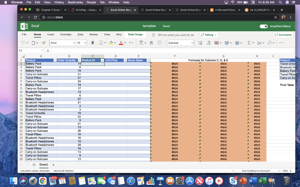
In the given spreadsheet, columns A though E represent a datatable. However, there are missing values in columns C through E. Incell J1 there is a lookup table containing columns for Product,Product ID, and Unit Price. Your first task is to fill in themissing values in columns C, D, and E using VLOOKUP and the lookuptable. Doing this manually would take a long time and be verytedious. The best way is to use VLOOKUP to fill in the first row ofmissing data and then drag down to fill the remaining rows.

In cell C2, populate the Product ID of the first item usingVLOOKUP. The value you wish to look up in the lookup table is inColumn A, cell A2 to be exact. The lookup table is cell range$J$1:$L$6. Note that these are absolute cell references since thelook up table is in a fixed location. The Product ID is in thesecond column of the lookup table. And finally set the range_lookupparameter to FALSE.

What is the Product ID returned in cell C2?

fill in the blank 2

Now repeat this process for the missing Unit Price in cell D2.What is the unit price returned in D2 (to the nearest cent)?

$fill in the blank 3

And finally, for the first item, calculate the Gross Sales incolumn E using Order Quantity from column B and Unit Price fromColumn D. What is the gross sale amount in cell E2?

$fill in the blank 4

To complete the data table, select cells C2, D2, and E2 togetherthen drag down or double-click the fill + sign in the lower rightof those three selected cells. And there you have it. The remaining147 items in columns C, D, and E have been completed using a lookuptable, two VLOOKUP formulas, a simple math formula, and Excel'sfill down feature.

Combining VLOOKUP with a Pivot Table

Now that you have the data table in columns A through E, a PivotTable can be used to summarize the data on a number of factors.

To create the Pivot Table, select the data in columns A throughE. Next, navigate to the Insert tab and click Pivot Table. Usingthe dialog box, place the Pivot Table in cell J10. Finally, usingthe Pivot Table Fields task pane on the right, create the PivotTable below and fill in the values.

NOTE: For the Sum of Gross Sales column, round answers tothe nearest cent and do not enter a dollar sign ($).

Row Labels	Sum of Order Quantity	Sum of Gross Sales ($)
Battery Pack	fill in the blank 5	$fill in the blank 6
Bluetooth Headphones	fill in the blank 7	$fill in the blank 8
Carry-on Suitcase	fill in the blank 9	$fill in the blank 10
Travel Pillow	fill in the blank 11	$fill in the blank 12
Travel Umbrella	fill in the blank 13	$fill in the blank 14
Grand Total	fill in the blank 15	$fill in the blank 16

Chrome File Edit View History Bookmarks People Tab Window Help ... th Chapter 2 Excel T XMindTap - Cenga x about:blank C X Excel File Dv C2 Home A 6 7 8 Battery Pack Insert 1 Product Battery Pack 2 3 Battery Pack 4 Battery Pack 5 Carry-on Suitcase Travel Pillow Carry-on Suitcase fx Travel Umbrella 9 Carry-on Suitcase 10 Bluetooth Headphones 11 Travel Pillow 12 Battery Pack 13 Bluetooth Headphones 14 Bluetooth Headphones 15 Bluetooth Headphones 16 17 Travel Pillow 18 Battery Pack 19 Carry-on Suitcase 20 Carry-on Suitcase 21 Carry-on Suitcase 22 Travel Pillow 23 Bluetooth Headphones Arial 24 Bluetooth Headphones 25 Bluetooth Headphones 26 Travel Pillow 27 Carry-on Suitcase 28 Carry-on Suitcase 29 Carry-on Suitcase = Sheet1 + Calculation Mode: Automatic Formulas 4,311, B Order Quantity Workbook Statistics 24 12 Data Review 10 14 8 19 21 27 24 19 17 13 6 27 21 3 3 19 22 9 21 13 26 10 16 15 29 18 13 9 13 Excel Online Stude X C Product ID View Help B D Unit Price 212 Table Design AV... template Excel Online Stude X E Gross Sales V 7 7 Saved Tell me what you want to do General F #N/A #N/A #N/A #N/A #N/A #N/A #N/A #N/A #N/A #N/A #N/A #N/A #N/A #N/A #N/A #N/A #N/A #N/A #N/A #N/A #N/A #N/A #N/A #N/A #N/A #N/A Excel Online Stude X #N/A #N/A O (A) Editing G Formulas for Columns C, D, & E #N/A #N/A #N/A #N/A #N/A #N/A #N/A #N/A #N/A #N/A #N/A F F F A Microsoft Excel X SO 0 #N/A #N/A #N/A #N/A #N/A #N/A #N/A #N/A #N/A #N/A #N/A 89% Fri 8:29 AM #N/A #N/A #N/A #N/A #N/A #N/A S CHE VLOOKUP Fun X P #N/A #N/A #N/A #N/A #N/A #N/A #N/A #N/A #N/A #N/A #N/A #N/A #N/A #N/A F H #N/A #N/A #N/A #N/A #N/A #N/A #N/A #N/A W #N/A #N/A Give Feedback to Microsoft #N/A #N/A #N/A #N/A X I Q + Simplified Ribbon 18 E Comments *** Product Travel Umbr Bluetooth H Battery Pack Travel Pillow Carry-on Su Pivot Table -100% +