these are the algorithms.

The algorithms are for this question.

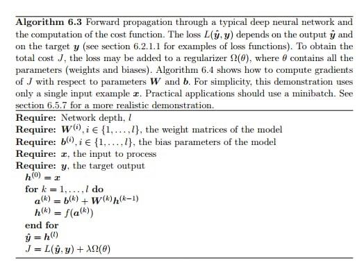
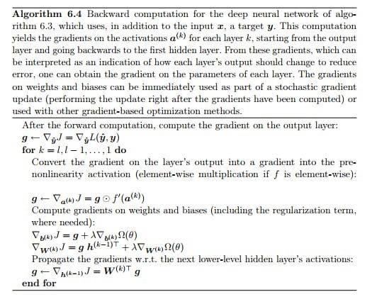
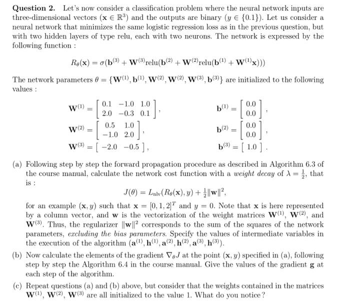
Algorithm 6.3 Forward propagation through a typical deep neural network and the computation of the cost function. The loss L,y) depends on the output y and on the target y (see section 6.2.1.1 for examples of loss functions). To obtain the total cost J, the loss may be added to a regularizer 12(0), where 8 contains all the parameters (weights and biases). Algorithm 6.4 shows how to compute gradients of J with respect to parameters W and b. For simplicity, this demonstration uses only a single input example 2. Practical applications should use a minibatch. See section 6.5.7 for a more realistic demonstration. Require: Network depth. I Require: W0i {1,...,1}, the weight matrices of the model Require: bli e {1.....l}, the bias parameters of the model Require: , the input to process Require: y, the target output h() = 1 for k = 1,...,/ do a) 6(k) + W(k) (k-1) h() = f(a(k)) end for y = 10) J = Ly, y) + AN(0) Algorithm 6.4 Backward computation for the deep neural network of algo- rithm 6.3, which uses, in addition to the input I, a target y. This computation yields the gradients on the activations a(k) for each layer k, starting from the output layer and going backwards to the first hidden layer. From these gradients, which can be interpreted as an indication of how each layer's output should change to reduce error, one can obtain the gradient on the parameters of each layer. The gradients on weights and biases can be immediately used as part of a stochastic gradient update (performing the update right after the gradients have been computed) or used with other gradient-based optimization methods. After the forward computation, compute the gradient on the output layer: 9-= V.y) for k=1,1-1,..., 1 do Convert the gradient on the layer's output into a gradient into the pre- nonlinearity activation (element-wise multiplication if f is element-wise): 9-X) J = go f'(a)) Compute gradients on weights and biases (including the regularization term, where needed): J = 9+2() wwJ=g ha-1)T + Xw2(0) Propagate the gradients w.r.t. the next lower-level hidden layer's activations: 9- hk-1) = WT 9 end for W(1) (1) 1.0 W(2) [ :] b) [ 0 ] + Question 2. Let's now consider a classification problem where the neural network inputs are three-dimensional vectors (x R) and the outputs are binary (y (0.1}). Let us consider a neural network that minimizes the same logistic regression loss as in the previous question, but with two hidden layers of type relu, each with two neurons. The network is expressed by the following function : Ry(x) = g(63) + Wrelu(b(2) + Wrelu(b() + W()); The network parameters 0 = {W(1), 6(1), (2), (2), 3), b)} are initialized to the following values: 0.1 -1.0 1.0 0.0 2.0 -0.3 0.1 0.0 0.5 0.0 -1.0 2.0 0.0 W(3) = [ -2.0 -0.5], b(3) = (1.0) (a) Following step by step the forward propagation procedure as described in Algorithm 6.3 of the course manual, calculate the network cost function with a weight decay of 1 = , that J(O) = Lnlv(R$(x), y) + 1 ||w|? for an example (x,y) such that x = [0,1, 2" and y = 0. Note that x is here represented by a column vector, and w is the vectorization of the weight matrices W(1), W(2), and W3). Thus, the regularizer || w || 2 corresponds to the sum of the squares of the network parameters, excluding the bias parameters. Specify the values of intermediate variables in the execution of the algorithm (a), h), a 2), h), a 3), h). (b) Now calculate the elements of the gradient VJ at the point (x, y) specified in (a), following step by step the Algorithm 6.4 in the course manual. Give the values of the gradient g at each step of the algorithm. (c) Repeat questions (a) and (b) above, but consider that the weights contained in the matrices W(1), W2), W(3) are all initialized to the value 1. What do you notice? Algorithm 6.3 Forward propagation through a typical deep neural network and the computation of the cost function. The loss L,y) depends on the output y and on the target y (see section 6.2.1.1 for examples of loss functions). To obtain the total cost J, the loss may be added to a regularizer 12(0), where 8 contains all the parameters (weights and biases). Algorithm 6.4 shows how to compute gradients of J with respect to parameters W and b. For simplicity, this demonstration uses only a single input example 2. Practical applications should use a minibatch. See section 6.5.7 for a more realistic demonstration. Require: Network depth. I Require: W0i {1,...,1}, the weight matrices of the model Require: bli e {1.....l}, the bias parameters of the model Require: , the input to process Require: y, the target output h() = 1 for k = 1,...,/ do a) 6(k) + W(k) (k-1) h() = f(a(k)) end for y = 10) J = Ly, y) + AN(0) Algorithm 6.4 Backward computation for the deep neural network of algo- rithm 6.3, which uses, in addition to the input I, a target y. This computation yields the gradients on the activations a(k) for each layer k, starting from the output layer and going backwards to the first hidden layer. From these gradients, which can be interpreted as an indication of how each layer's output should change to reduce error, one can obtain the gradient on the parameters of each layer. The gradients on weights and biases can be immediately used as part of a stochastic gradient update (performing the update right after the gradients have been computed) or used with other gradient-based optimization methods. After the forward computation, compute the gradient on the output layer: 9-= V.y) for k=1,1-1,..., 1 do Convert the gradient on the layer's output into a gradient into the pre- nonlinearity activation (element-wise multiplication if f is element-wise): 9-X) J = go f'(a)) Compute gradients on weights and biases (including the regularization term, where needed): J = 9+2() wwJ=g ha-1)T + Xw2(0) Propagate the gradients w.r.t. the next lower-level hidden layer's activations: 9- hk-1) = WT 9 end for W(1) (1) 1.0 W(2) [ :] b) [ 0 ] + Question 2. Let's now consider a classification problem where the neural network inputs are three-dimensional vectors (x R) and the outputs are binary (y (0.1}). Let us consider a neural network that minimizes the same logistic regression loss as in the previous question, but with two hidden layers of type relu, each with two neurons. The network is expressed by the following function : Ry(x) = g(63) + Wrelu(b(2) + Wrelu(b() + W()); The network parameters 0 = {W(1), 6(1), (2), (2), 3), b)} are initialized to the following values: 0.1 -1.0 1.0 0.0 2.0 -0.3 0.1 0.0 0.5 0.0 -1.0 2.0 0.0 W(3) = [ -2.0 -0.5], b(3) = (1.0) (a) Following step by step the forward propagation procedure as described in Algorithm 6.3 of the course manual, calculate the network cost function with a weight decay of 1 = , that J(O) = Lnlv(R$(x), y) + 1 ||w|? for an example (x,y) such that x = [0,1, 2" and y = 0. Note that x is here represented by a column vector, and w is the vectorization of the weight matrices W(1), W(2), and W3). Thus, the regularizer || w || 2 corresponds to the sum of the squares of the network parameters, excluding the bias parameters. Specify the values of intermediate variables in the execution of the algorithm (a), h), a 2), h), a 3), h). (b) Now calculate the elements of the gradient VJ at the point (x, y) specified in (a), following step by step the Algorithm 6.4 in the course manual. Give the values of the gradient g at each step of the algorithm. (c) Repeat questions (a) and (b) above, but consider that the weights contained in the matrices W(1), W2), W(3) are all initialized to the value 1. What do you notice