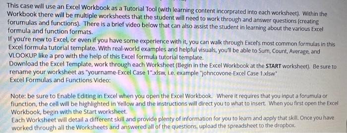
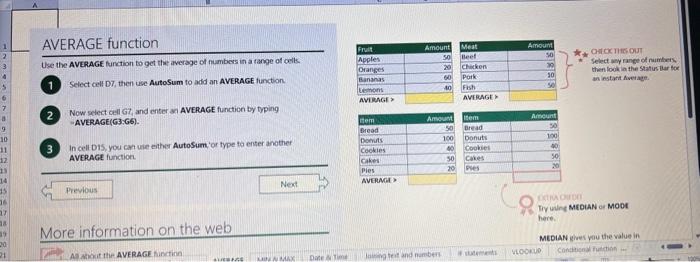
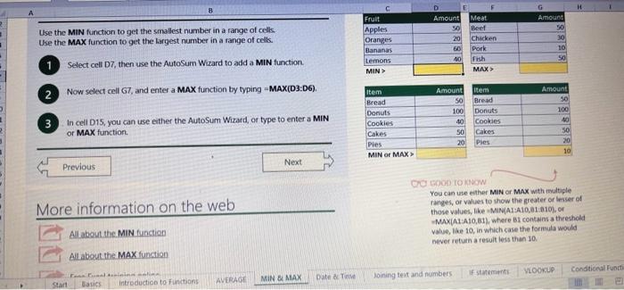
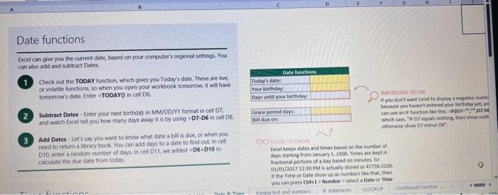
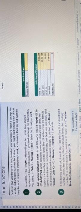
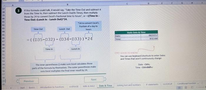
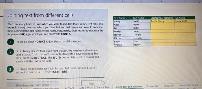
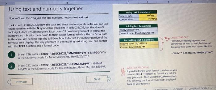
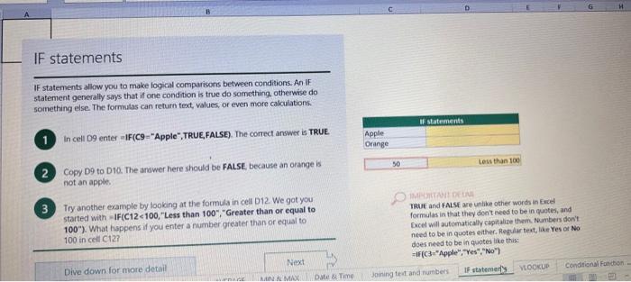
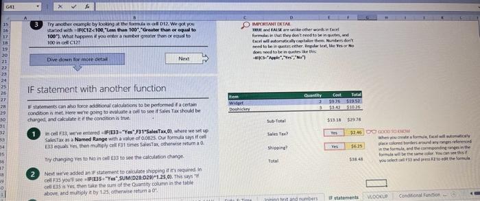
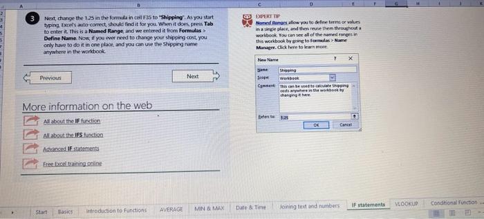
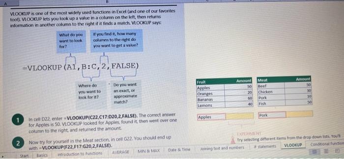
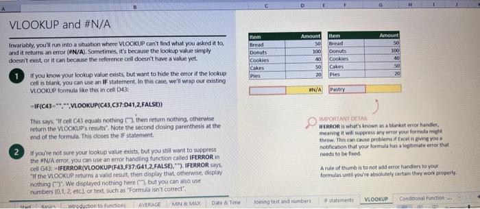
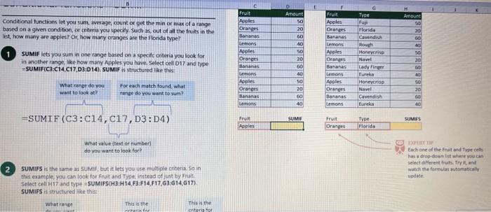
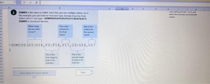
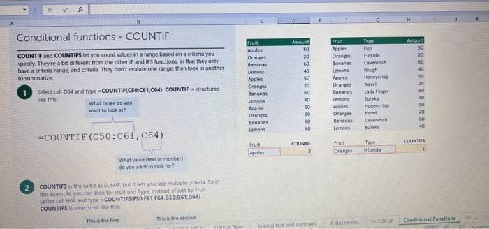
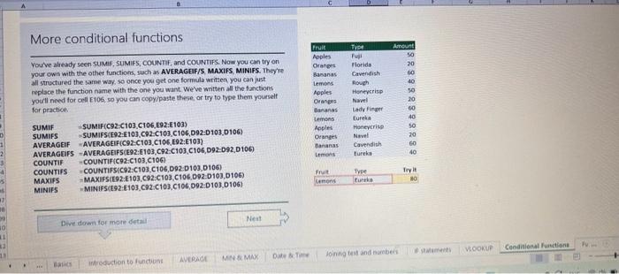
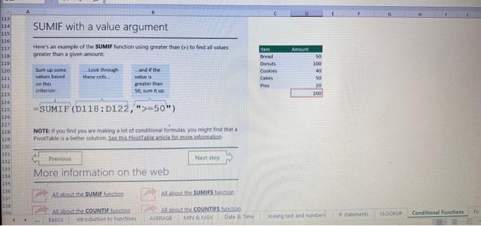
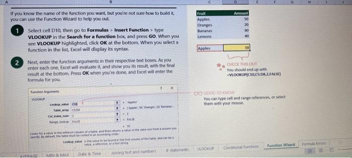
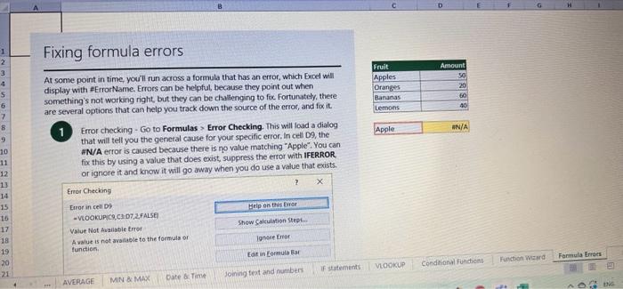
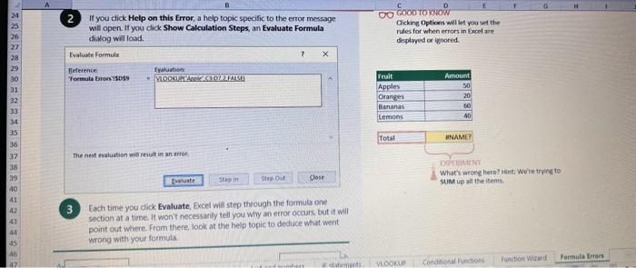
This case will use an Excel Workbook as a Tutorial Tool (with learning content incorprated into each worksheet). Within the Workbook there will be multiple worksheets that the student will need to work through and answer questions (creating forumulas and functions). There is a brief video below that can also assist the student in learning about the various Excel formula and function formats. If you're new to Excel, or even if you have some experience with it, you can walk through Excel's most common formulas in this Excel formula tutorial template. With real-world examples and helpful visuals, you'll be able to Sum, Count, Average, and VLOOKUP like a pro with the help of this Excel formula tutorial template. Download the Excel Template, work through each Worksheet (Begin in the Excel Workbook at the START worksheet). Be sure to rename your worksheet as "yourname-Excel Case 1".xIsw, i.e. example "johncovone-Excel Case 1.xlsw" Excel Formulas and Functions Video: Note: be sure to Enable Editing in Excel when you open the Excel Workbook. Where it requires that you input a forumula or fiunction, the cell will be highlighted in Yellow and the instructions will direct you to what to insert. When you first open the Excel Workbook, begin with the Start worksheet. Each Worksheet will detail a different skill and provide plenty of information for you to learn and apply that skill, Once you have worked through all the Worksheets and answered all of the questions, upload the spreadsheet to the dropbox. Use the AVERAGE turution to get the average of fumbers in a famge of odk- Select cell DT, then use AutoSum to add an AVERAGE function. Now select cill GZ, and enter aA AVERACE function by fyping AVERAGE(G3,G6). In cell Dis. you cart uie eitws AutoSum,'or type to enter another Averace function More information on the web Tiy usir stsotaN or Mabt hare. Use the MIN function to get the smallest number in a range of cells Use the MAX function to get the largest number in a range of cells. Select cell D7, then use the AutoSum Wizard to add a MIN function. Now select cell G7, and enter a MAX function by typing = MAX(D3:D6). In cell D15, you can use either the AutoSum Wizard, or type to enter a MIN or MAX function. More information on the web You can use eather MuN or Max wath multiple ranges, or values to show the freater or lenser of those values, like imimaratio, a1: 010 , or Allabout the Min function - Max(A1:A10,B1), where B1 contains a threshold value, like 10, in which case the formula would Allabout the MAX function Excel can give you the current date, based on your computer's regional settings You can also add and subtract Dates. Oheck out the TODAY function, which gives you Today's date. These are live. or volatie functions, s0 when you apen your workbock tomortow, it will have tomorrows date. Enter eTODAYO in cell D6. Subtract Dates - Enter your next birthday in MMDDMY format in cell D7. and watch Excel tell you how many days awoy it is by using = D7.-D6 in celt D8. Add Dates - Lef's say you want to know what date a bili is due, of when you fneed to return a library book. You can add days to a date to find out, in cel D10, enter a random number of dsys, In cell 011, we added = D6.D10 to calculate the dive date from today, Dreel keeps idates and times based on the number of ders starting from laruary 1, 1900. Times are lept in fractionad portions of a dey based on minutes 50 If the Time or Dase thow up as numbers like that, then you cen press Culet > Namber s select a bate or Time Fecel can give you the current time, based on your computer's regional setlings. You can also add and subtract times. For instance you might need to keep track of how marry hours an employe worked each week, and calculate their pay and overtime 1 In cell 028 enter = NOWO, which will give the current time, and will update each time Excel calculates, if you need to change the Time format. you can 90 to Ctrl+1>. Number > Time > Select the fotmat you want. 2 Add up hours between times - In cell D36 we've entered w((D35.D32) (D34-D33))'24, which calculates someone's start and end finmes, then subracts the time they took for lunch. The 224 at the end of the formula corverts the fractional portion of the day that Excel sees into hours. Youil need to format the cell as a Number though. To do that go to Home : Format > Cells (Ctri+1)> Number > Number >2 decimals: 3. If thin formula could tak, it would say, "Tane the fime Out and rubtract a from the Time in then sudtract the tunch Out/in Times, then ifwitiply those by 24 to convert Ercels frational time to hour";, or "(Time In Time Out)-(tunch in - Lunch Out)) 224 . 724 to convert Lucefa If this formula could talk, it would say, Take the Time out and subtrnct it from the Time in, then subtract the Lunch Out Times, then multiply thase by 24 to cosivert Excel's fractional time to hours; or = (CTime In Time Out)-(Lunch In - Lunch Out) )24. You can use keyboard shortcuts to enter Dutes and Times that wont continuously thinge: The inrer parentheser () make sure excen cescuiatos unm Date - Curle: parts of the formula by themselves. The cuter parentheses make Time ctritshifte: sure Dxcel multiplies the final inner result by 24 . Joining text from different cells There are many times in Excel when you want to join text that's in different cells. This: example is very common, where you have first and last names, and want to combine them as first name, last name, or full name. Fortunately, Excel lets us do that with the Arnpersand (82) sign, which you can enter with Shift +7. In cell E3, enter =D38C3 to join the last and first farmes. SmithNancy doesn't look quite right though. We need to add a comma and a space. To do that we il use quotes to create a new text string. This: time, enter = D38", "giC3. The 8x, " portion lets us join a corama and space with the text in the celis. To create the full name, we'll join first and last name, but use a space Now we'il use the & to join text and numbers, not just text and text Look at cells C288D29. See how the date and times are in separate cells? You can join them together with the 8 symbol like you'll see in cells C3233, but that doesi't look right, does it? Unfortunately, Excel doesn't know how you want to format the numbers, so it breaks them down to their basest format, which is the the Setial date in this case. We need to explicity tell Excel how to format the number portion of the formula, so it displays the way you want in the resulting text string. You can do that with the TEXT function and a format code. In cell C36, enter = C288" - gTEXT(D28, "MM/DD/YYYY"). MM/DD/YYY is the US format code for MontlVDay/Year, like 09/25/2017. In cell C37, enter = C298" " \&TEXT(D29, "HH:MM AM/PM"). HMM AM/PM is the US format code for Hours Minutes AM or PM, like 1:30 PM. If you don't know what format code to use, you can we ctrtit > Number to format any cell the way you want. Then select the Custom option. You can copy the formut code that's displayed back to your formula. If staternents allow you to make logical comparisons between conditions. An If statement generally says that if one condition is true do something, otherwise do something else. The formulas can return text, values, of even more calculations. In cell D9 enter =IF(C9="Apple", TRUE, FALSE). The conrect answer is TRUE. Copy D9 to D10. The answer here should be FALSE, because an orange is not an apple. Try another example by looking at the formula in cell D12. We got you started with = IF(C12100," Greater than or equal to 100 ). What happens if you enter a number greater than or equal to 100 in cell Cl2? Inde and falst are untike other words in Excel. formulas in that they don' need to be in quotes, and frcel will automatically capitalize them. Numbers don't. need to be in quotes either. Regular test, like Yes or No does need to be in quotes like this: =if(c3-"Apple", "Yes","No") (3) Try another example by kooting at the formine in oill o12 We got you stated with = Ific12F33, weve entered affiB33 - 'Yes", F31'Saleitax 0 , where we set up Salestax as 2 Named Range with a value of o. ovis, Our formula shys if cel E3 equals ves. then multiply cell fat times siestax otherwive retum a a Try changing yer to No in cel Ea3 to see the calculabise chabge. Next we've added an if statement to calculare shpping it irs moured in cell F35 you wee - IF(E35 - 'Yes", sum (D22-D29)"1.25, 09, this sys of cell E35 is Yes, then take the sum of the Cuantity cosmen in the table. above, and murichy it by 125 , otherwice cotum a of. (3) Next, dange the 1.25 in the formula in cell F3s to "Shipping". As you start typing bxcels aito correct, should find it for you. When it does, press Tab to enter it, This is a Named Flange and we entered if from Formulas ? Define Name Now, if you env need to diange your shipping cost you in a sirge ploce, and then reve them thenuchout a only have to do in one place, and you can use the Shipping rame this weribook thy ghing to femmalar > Name. ampohere in the workbock: Manden. Click here to licarn more More information on the web Allabout the IF furstion Allabout the IfS futition Atvanced if gutements Frse Froci training oroling VLOOKUP is one of the most widely used functions in Excel fand one of our favonites tool). VLOOKUP lets you look up a value in a column on the left, then returns infomation in another column to the right if it finds a match. VLOOKUP says: 1 In cell D22, enter = VLOOKUP(C22,C17:D20,2,FALSE). The correct answer: for Apples is 50. VLOOKUP looked for Apples, found it, then went over one column to the right, and returned the amount. Invariably, you'l run into a situation where vLOOKUP can't find what you asked it to. and it returns an error (NN/A). Socnetimes, it's because the lookup value simply doesn't exist, or it can because the reference cell doesn't have a value yet. 1 If you know your lookup value exists, but want to hide the error if the lookup cell is blank, you can use an If statement. In this case, well wrap our existing VLOOKUP formula like this in celi D43: = IF(C43 = *,", VLOOKUP(C43,C37:D41,2,FALSE)) This says, 7 cell C4.3 equats nothing (7, then retuin nothing, otherwise return the VLOOKUP's results:. Note the second closing parenthesis at the end of the formula. This coses the If statement. 2. If you're not sure your lookup value exists, but you still want to suppress the UN/A error, you can use an error handling function called IFERROR in cell G43: - IFERROR(VLOOKUP(F43, F37:G41,2, FALSE). "). IFERROR says. "If the VLOOKUP returns a valid result, then dispiay that, otherwise, display nothing ("). We displayed nothing here ("), but you can also use numbers (0,1,2, etc), or text, such as "Formula isnt correct". Conditional functions let you sum average, werk or get the min or max of a range based on a grven condition, or criteria you specily. Such as, out of all the frits in the list, how many are applest Or, how marty oranges are the Flonida type? 1. SUMIF lets you sum in one range based on a specitc criteria you bok for in another range, like how many Apples you have. Select oell DiT and type - SUMIF(C3.C14,C17, D3:014), SUMIF is structured like this: 2 SUMiFS is the mame as SUlaif, but it lets you use multple criteria. So in this erample, you can look for Frilt and Typt, inatead of just by Fruat. Select cell H17 and type w sUMiFS(H3:H14, F3.F14, F17, G3.G14,G17) SUMIFS is structured like this: SUMIFS is the same is SUMEF, but it ketr you use multiple chiteria. So in this example, you can look for Finit and Type, instead of just by finat, Solect cebHi7 and type n\$UMIFS(H3:H14,F3:F14, F17, G3.614, G17). SUMIFS is structured like thes: COUNTIF and COUNTIFS let you count values in a range based on a cititeria you specity. Theyre a bit different from the other if and ifs functions, in that they only have a criteria range, and criteria. They dont evalute one range, then look in anothet to summarize. 1 Select cell D64 and type = COUNTIF(CS0,C61, C64). COUNTIF is structured What value (text or number) do you zant to look for? COUNTIFS in the same as sUMis, but it lets you use multiple critecia. 50 in this example, you can look foc fruit and Type, initead of just by Friat. Select cell H54 and type = COUNTIFS(FSO.F61,F64,GSO.G61,G64). COUNTIFS is structured the thil: More conditional functions You've already secn SUMif, 5UMIFS, COUNTII, and CouUNTIFS. Now you ean try on your own with the other functioers, such a AVERAGEIF/S. MAXIFS. MINIFS. Theyre all structured the same way, so once you get one tormula writsen you can just replace the function name with the one you want. We've written all the functions yourll need for cell E106, so you can copydpaste these, or try to bype them yourself for practicoi. SUMIF with a value argument Here's an coample of the SUMIF function using greater than (>) to find all values greaser than a given amount: =SUMIF(D118:D122,>50n) NOTE: if you find you are making a lot of conditional formulas you might find that a If you know the name of the function you want, but you're not sure how to build it, you can use the Function Wizard to help you out. 1. Select cell D10, then go to Formulas > Insert Function > type VLOOKUP in the Search for a function box, and press GO. When you see VLOOKUP highlighted, click OK at the bottom. When you select a function in the list, Excel will display its syntax. Next, enter the function arguments in their respective text boxes, As you enter each one. Excel will evaluate it, and show you its result, with the final result at the bottom. Press OK when you're done, and Excel will enter the formula for you. You should end up with -vioosuric10,CS:08,2.FAist) You can type cell and range referseces, or select them with your mouse. At some point in time, you'll run across a formula that has an error, which Excel will display with *ErrorName. Errecs can be helphul, because they point out when something's not working right, but thcy can be challenging to foc. Fortunately, there are several options that can help you track down the source of the error, and fox it. Error checking - Go to Formulas > Error Checking. This will load a dialog that will tell you the general cause for your specific error, In cell D9, the \#N/A error is caused because there is no value matching "Apple"; You can fix this by using a value that does exist, suppress the error with IFERROR. or ignore it and know it will go away when you do use a value that exists. If you click Help on this Error, a help topic specific to the error message will open. If you click Show Calculation Steps, an Evaluate Formula Cicking Options will let you wet the dialog will lood. rules for when errors in Excel are isciplyed or ignored. Evaluate Formula fleference Fraluabser Fermula Enarstsisse The neit rualuation will reut in an errer, 3. Fach time you cick Evaluate, Excel will step through the formula one section at a time. If won't necessarly tell you wity an error occurs, but it will point out where. from there, look at the help topic to decduce what went wrong with your formula. This case will use an Excel Workbook as a Tutorial Tool (with learning content incorprated into each worksheet). Within the Workbook there will be multiple worksheets that the student will need to work through and answer questions (creating forumulas and functions). There is a brief video below that can also assist the student in learning about the various Excel formula and function formats. If you're new to Excel, or even if you have some experience with it, you can walk through Excel's most common formulas in this Excel formula tutorial template. With real-world examples and helpful visuals, you'll be able to Sum, Count, Average, and VLOOKUP like a pro with the help of this Excel formula tutorial template. Download the Excel Template, work through each Worksheet (Begin in the Excel Workbook at the START worksheet). Be sure to rename your worksheet as "yourname-Excel Case 1".xIsw, i.e. example "johncovone-Excel Case 1.xlsw" Excel Formulas and Functions Video: Note: be sure to Enable Editing in Excel when you open the Excel Workbook. Where it requires that you input a forumula or fiunction, the cell will be highlighted in Yellow and the instructions will direct you to what to insert. When you first open the Excel Workbook, begin with the Start worksheet. Each Worksheet will detail a different skill and provide plenty of information for you to learn and apply that skill, Once you have worked through all the Worksheets and answered all of the questions, upload the spreadsheet to the dropbox. Use the AVERAGE turution to get the average of fumbers in a famge of odk- Select cell DT, then use AutoSum to add an AVERAGE function. Now select cill GZ, and enter aA AVERACE function by fyping AVERAGE(G3,G6). In cell Dis. you cart uie eitws AutoSum,'or type to enter another Averace function More information on the web Tiy usir stsotaN or Mabt hare. Use the MIN function to get the smallest number in a range of cells Use the MAX function to get the largest number in a range of cells. Select cell D7, then use the AutoSum Wizard to add a MIN function. Now select cell G7, and enter a MAX function by typing = MAX(D3:D6). In cell D15, you can use either the AutoSum Wizard, or type to enter a MIN or MAX function. More information on the web You can use eather MuN or Max wath multiple ranges, or values to show the freater or lenser of those values, like imimaratio, a1: 010 , or Allabout the Min function - Max(A1:A10,B1), where B1 contains a threshold value, like 10, in which case the formula would Allabout the MAX function Excel can give you the current date, based on your computer's regional settings You can also add and subtract Dates. Oheck out the TODAY function, which gives you Today's date. These are live. or volatie functions, s0 when you apen your workbock tomortow, it will have tomorrows date. Enter eTODAYO in cell D6. Subtract Dates - Enter your next birthday in MMDDMY format in cell D7. and watch Excel tell you how many days awoy it is by using = D7.-D6 in celt D8. Add Dates - Lef's say you want to know what date a bili is due, of when you fneed to return a library book. You can add days to a date to find out, in cel D10, enter a random number of dsys, In cell 011, we added = D6.D10 to calculate the dive date from today, Dreel keeps idates and times based on the number of ders starting from laruary 1, 1900. Times are lept in fractionad portions of a dey based on minutes 50 If the Time or Dase thow up as numbers like that, then you cen press Culet > Namber s select a bate or Time Fecel can give you the current time, based on your computer's regional setlings. You can also add and subtract times. For instance you might need to keep track of how marry hours an employe worked each week, and calculate their pay and overtime 1 In cell 028 enter = NOWO, which will give the current time, and will update each time Excel calculates, if you need to change the Time format. you can 90 to Ctrl+1>. Number > Time > Select the fotmat you want. 2 Add up hours between times - In cell D36 we've entered w((D35.D32) (D34-D33))'24, which calculates someone's start and end finmes, then subracts the time they took for lunch. The 224 at the end of the formula corverts the fractional portion of the day that Excel sees into hours. Youil need to format the cell as a Number though. To do that go to Home : Format > Cells (Ctri+1)> Number > Number >2 decimals: 3. If thin formula could tak, it would say, "Tane the fime Out and rubtract a from the Time in then sudtract the tunch Out/in Times, then ifwitiply those by 24 to convert Ercels frational time to hour";, or "(Time In Time Out)-(tunch in - Lunch Out)) 224 . 724 to convert Lucefa If this formula could talk, it would say, Take the Time out and subtrnct it from the Time in, then subtract the Lunch Out Times, then multiply thase by 24 to cosivert Excel's fractional time to hours; or = (CTime In Time Out)-(Lunch In - Lunch Out) )24. You can use keyboard shortcuts to enter Dutes and Times that wont continuously thinge: The inrer parentheser () make sure excen cescuiatos unm Date - Curle: parts of the formula by themselves. The cuter parentheses make Time ctritshifte: sure Dxcel multiplies the final inner result by 24 . Joining text from different cells There are many times in Excel when you want to join text that's in different cells. This: example is very common, where you have first and last names, and want to combine them as first name, last name, or full name. Fortunately, Excel lets us do that with the Arnpersand (82) sign, which you can enter with Shift +7. In cell E3, enter =D38C3 to join the last and first farmes. SmithNancy doesn't look quite right though. We need to add a comma and a space. To do that we il use quotes to create a new text string. This: time, enter = D38", "giC3. The 8x, " portion lets us join a corama and space with the text in the celis. To create the full name, we'll join first and last name, but use a space Now we'il use the & to join text and numbers, not just text and text Look at cells C288D29. See how the date and times are in separate cells? You can join them together with the 8 symbol like you'll see in cells C3233, but that doesi't look right, does it? Unfortunately, Excel doesn't know how you want to format the numbers, so it breaks them down to their basest format, which is the the Setial date in this case. We need to explicity tell Excel how to format the number portion of the formula, so it displays the way you want in the resulting text string. You can do that with the TEXT function and a format code. In cell C36, enter = C288" - gTEXT(D28, "MM/DD/YYYY"). MM/DD/YYY is the US format code for MontlVDay/Year, like 09/25/2017. In cell C37, enter = C298" " \&TEXT(D29, "HH:MM AM/PM"). HMM AM/PM is the US format code for Hours Minutes AM or PM, like 1:30 PM. If you don't know what format code to use, you can we ctrtit > Number to format any cell the way you want. Then select the Custom option. You can copy the formut code that's displayed back to your formula. If staternents allow you to make logical comparisons between conditions. An If statement generally says that if one condition is true do something, otherwise do something else. The formulas can return text, values, of even more calculations. In cell D9 enter =IF(C9="Apple", TRUE, FALSE). The conrect answer is TRUE. Copy D9 to D10. The answer here should be FALSE, because an orange is not an apple. Try another example by looking at the formula in cell D12. We got you started with = IF(C12100," Greater than or equal to 100 ). What happens if you enter a number greater than or equal to 100 in cell Cl2? Inde and falst are untike other words in Excel. formulas in that they don' need to be in quotes, and frcel will automatically capitalize them. Numbers don't. need to be in quotes either. Regular test, like Yes or No does need to be in quotes like this: =if(c3-"Apple", "Yes","No") (3) Try another example by kooting at the formine in oill o12 We got you stated with = Ific12F33, weve entered affiB33 - 'Yes", F31'Saleitax 0 , where we set up Salestax as 2 Named Range with a value of o. ovis, Our formula shys if cel E3 equals ves. then multiply cell fat times siestax otherwive retum a a Try changing yer to No in cel Ea3 to see the calculabise chabge. Next we've added an if statement to calculare shpping it irs moured in cell F35 you wee - IF(E35 - 'Yes", sum (D22-D29)"1.25, 09, this sys of cell E35 is Yes, then take the sum of the Cuantity cosmen in the table. above, and murichy it by 125 , otherwice cotum a of. (3) Next, dange the 1.25 in the formula in cell F3s to "Shipping". As you start typing bxcels aito correct, should find it for you. When it does, press Tab to enter it, This is a Named Flange and we entered if from Formulas ? Define Name Now, if you env need to diange your shipping cost you in a sirge ploce, and then reve them thenuchout a only have to do in one place, and you can use the Shipping rame this weribook thy ghing to femmalar > Name. ampohere in the workbock: Manden. Click here to licarn more More information on the web Allabout the IF furstion Allabout the IfS futition Atvanced if gutements Frse Froci training oroling VLOOKUP is one of the most widely used functions in Excel fand one of our favonites tool). VLOOKUP lets you look up a value in a column on the left, then returns infomation in another column to the right if it finds a match. VLOOKUP says: 1 In cell D22, enter = VLOOKUP(C22,C17:D20,2,FALSE). The correct answer: for Apples is 50. VLOOKUP looked for Apples, found it, then went over one column to the right, and returned the amount. Invariably, you'l run into a situation where vLOOKUP can't find what you asked it to. and it returns an error (NN/A). Socnetimes, it's because the lookup value simply doesn't exist, or it can because the reference cell doesn't have a value yet. 1 If you know your lookup value exists, but want to hide the error if the lookup cell is blank, you can use an If statement. In this case, well wrap our existing VLOOKUP formula like this in celi D43: = IF(C43 = *,", VLOOKUP(C43,C37:D41,2,FALSE)) This says, 7 cell C4.3 equats nothing (7, then retuin nothing, otherwise return the VLOOKUP's results:. Note the second closing parenthesis at the end of the formula. This coses the If statement. 2. If you're not sure your lookup value exists, but you still want to suppress the UN/A error, you can use an error handling function called IFERROR in cell G43: - IFERROR(VLOOKUP(F43, F37:G41,2, FALSE). "). IFERROR says. "If the VLOOKUP returns a valid result, then dispiay that, otherwise, display nothing ("). We displayed nothing here ("), but you can also use numbers (0,1,2, etc), or text, such as "Formula isnt correct". Conditional functions let you sum average, werk or get the min or max of a range based on a grven condition, or criteria you specily. Such as, out of all the frits in the list, how many are applest Or, how marty oranges are the Flonida type? 1. SUMIF lets you sum in one range based on a specitc criteria you bok for in another range, like how many Apples you have. Select oell DiT and type - SUMIF(C3.C14,C17, D3:014), SUMIF is structured like this: 2 SUMiFS is the mame as SUlaif, but it lets you use multple criteria. So in this erample, you can look for Frilt and Typt, inatead of just by Fruat. Select cell H17 and type w sUMiFS(H3:H14, F3.F14, F17, G3.G14,G17) SUMIFS is structured like this: SUMIFS is the same is SUMEF, but it ketr you use multiple chiteria. So in this example, you can look for Finit and Type, instead of just by finat, Solect cebHi7 and type n\$UMIFS(H3:H14,F3:F14, F17, G3.614, G17). SUMIFS is structured like thes: COUNTIF and COUNTIFS let you count values in a range based on a cititeria you specity. Theyre a bit different from the other if and ifs functions, in that they only have a criteria range, and criteria. They dont evalute one range, then look in anothet to summarize. 1 Select cell D64 and type = COUNTIF(CS0,C61, C64). COUNTIF is structured What value (text or number) do you zant to look for? COUNTIFS in the same as sUMis, but it lets you use multiple critecia. 50 in this example, you can look foc fruit and Type, initead of just by Friat. Select cell H54 and type = COUNTIFS(FSO.F61,F64,GSO.G61,G64). COUNTIFS is structured the thil: More conditional functions You've already secn SUMif, 5UMIFS, COUNTII, and CouUNTIFS. Now you ean try on your own with the other functioers, such a AVERAGEIF/S. MAXIFS. MINIFS. Theyre all structured the same way, so once you get one tormula writsen you can just replace the function name with the one you want. We've written all the functions yourll need for cell E106, so you can copydpaste these, or try to bype them yourself for practicoi. SUMIF with a value argument Here's an coample of the SUMIF function using greater than (>) to find all values greaser than a given amount: =SUMIF(D118:D122,>50n) NOTE: if you find you are making a lot of conditional formulas you might find that a If you know the name of the function you want, but you're not sure how to build it, you can use the Function Wizard to help you out. 1. Select cell D10, then go to Formulas > Insert Function > type VLOOKUP in the Search for a function box, and press GO. When you see VLOOKUP highlighted, click OK at the bottom. When you select a function in the list, Excel will display its syntax. Next, enter the function arguments in their respective text boxes, As you enter each one. Excel will evaluate it, and show you its result, with the final result at the bottom. Press OK when you're done, and Excel will enter the formula for you. You should end up with -vioosuric10,CS:08,2.FAist) You can type cell and range referseces, or select them with your mouse. At some point in time, you'll run across a formula that has an error, which Excel will display with *ErrorName. Errecs can be helphul, because they point out when something's not working right, but thcy can be challenging to foc. Fortunately, there are several options that can help you track down the source of the error, and fox it. Error checking - Go to Formulas > Error Checking. This will load a dialog that will tell you the general cause for your specific error, In cell D9, the \#N/A error is caused because there is no value matching "Apple"; You can fix this by using a value that does exist, suppress the error with IFERROR. or ignore it and know it will go away when you do use a value that exists. If you click Help on this Error, a help topic specific to the error message will open. If you click Show Calculation Steps, an Evaluate Formula Cicking Options will let you wet the dialog will lood. rules for when errors in Excel are isciplyed or ignored. Evaluate Formula fleference Fraluabser Fermula Enarstsisse The neit rualuation will reut in an errer, 3. Fach time you cick Evaluate, Excel will step through the formula one section at a time. If won't necessarly tell you wity an error occurs, but it will point out where. from there, look at the help topic to decduce what went wrong with your formula