This code is for MATLAB. It requires the code and 3 plots for the data

Example template code

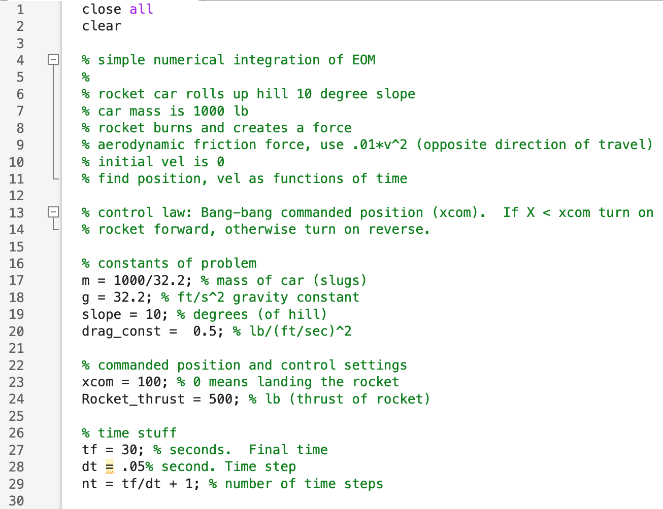
close all

clear

% simple numerical integration of EOM

%

% rocket car rolls up hill 10 degree slope

% car mass is 1000 lb

% rocket burns and creates a force

% aerodynamic friction force, use .01*v^2 (opposite direction of travel)

% initial vel is 0

% find position, vel as functions of time

% control law: Bang-bang commanded position (xcom). If X

% rocket forward, otherwise turn on reverse.

% constants of problem

m = 1000/32.2; % mass of car (slugs)

g = 32.2; % ft/s^2 gravity constant

slope = 10; % degrees (of hill)

drag_const = 0.5; % lb/(ft/sec)^2

% commanded position and control settings

xcom = 100; % 0 means landing the rocket

Rocket_thrust = 500; % lb (thrust of rocket)

% time stuff

tf = 30; % seconds. Final time

dt = .05% second. Time step

nt = tf/dt + 1; % number of time steps

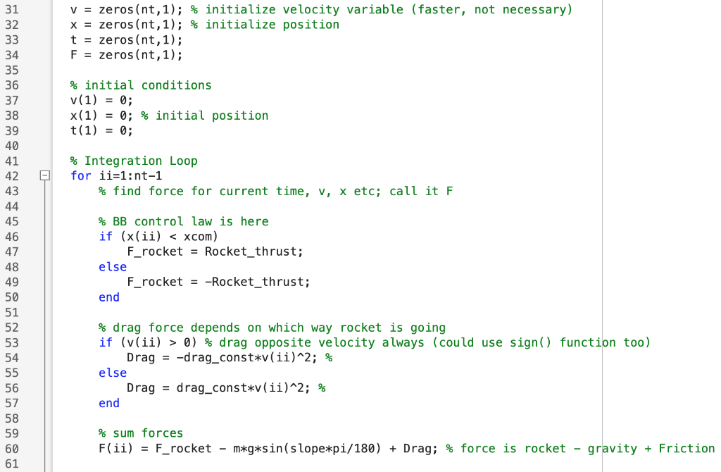
v = zeros(nt,1); % initialize velocity variable (faster, not necessary)

x = zeros(nt,1); % initialize position

t = zeros(nt,1);

F = zeros(nt,1);

% initial conditions

v(1) = 0;

x(1) = 0; % initial position

t(1) = 0;

% Integration Loop

for ii=1:nt-1

% find force for current time, v, x etc; call it F

% BB control law is here

if (x(ii)

F_rocket = Rocket_thrust;

else

F_rocket = -Rocket_thrust;

end

% drag force depends on which way rocket is going

if (v(ii) > 0) % drag opposite velocity always (could use sign() function too)

Drag = -drag_const*v(ii)^2; %

else

Drag = drag_const*v(ii)^2; %

end

% sum forces

F(ii) = F_rocket - m*g*sin(slope*pi/180) + Drag; % force is rocket - gravity + Friction

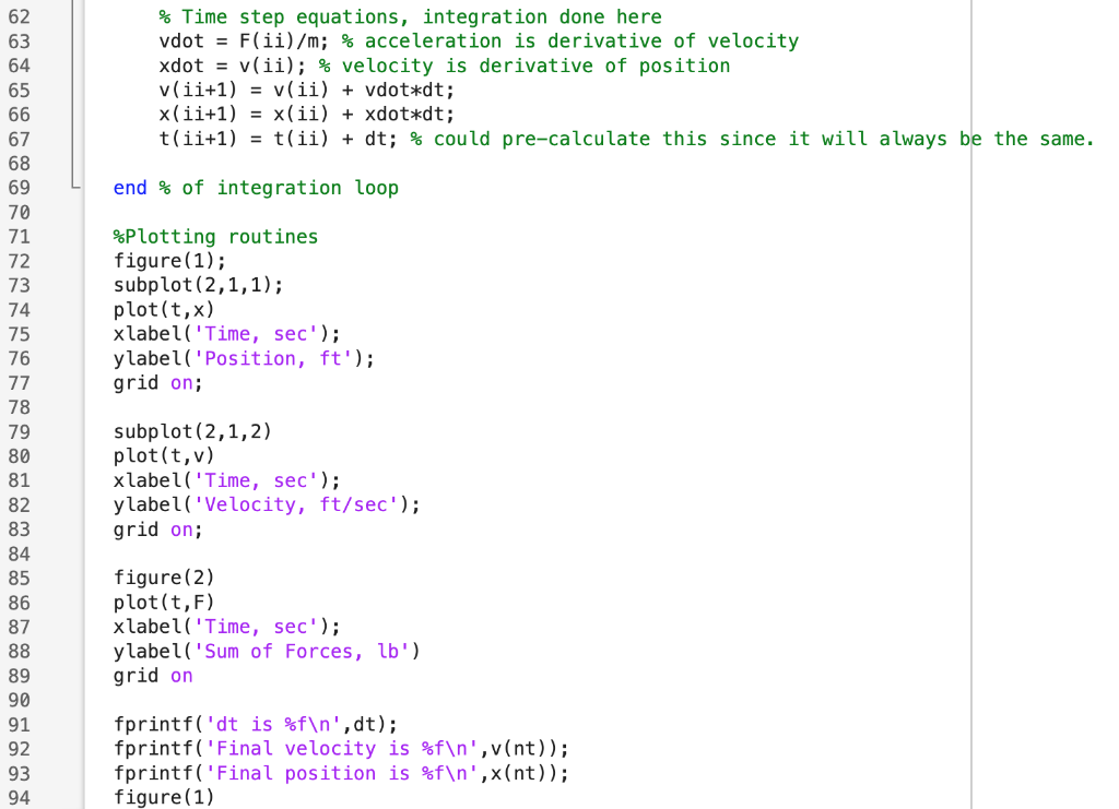
% Time step equations, integration done here

vdot = F(ii)/m; % acceleration is derivative of velocity

xdot = v(ii); % velocity is derivative of position

v(ii+1) = v(ii) + vdot*dt;

x(ii+1) = x(ii) + xdot*dt;

t(ii+1) = t(ii) + dt; % could pre-calculate this since it will always be the same.

end % of integration loop

%Plotting routines

figure(1);

subplot(2,1,1);

plot(t,x)

xlabel('Time, sec');

ylabel('Position, ft');

grid on;

subplot(2,1,2)

plot(t,v)

xlabel('Time, sec');

ylabel('Velocity, ft/sec');

grid on;

figure(2)

plot(t,F)

xlabel('Time, sec');

ylabel('Sum of Forces, lb')

grid on

fprintf('dt is %f ',dt);

fprintf('Final velocity is %f ',v(nt));

fprintf('Final position is %f ',x(nt));

figure(1)

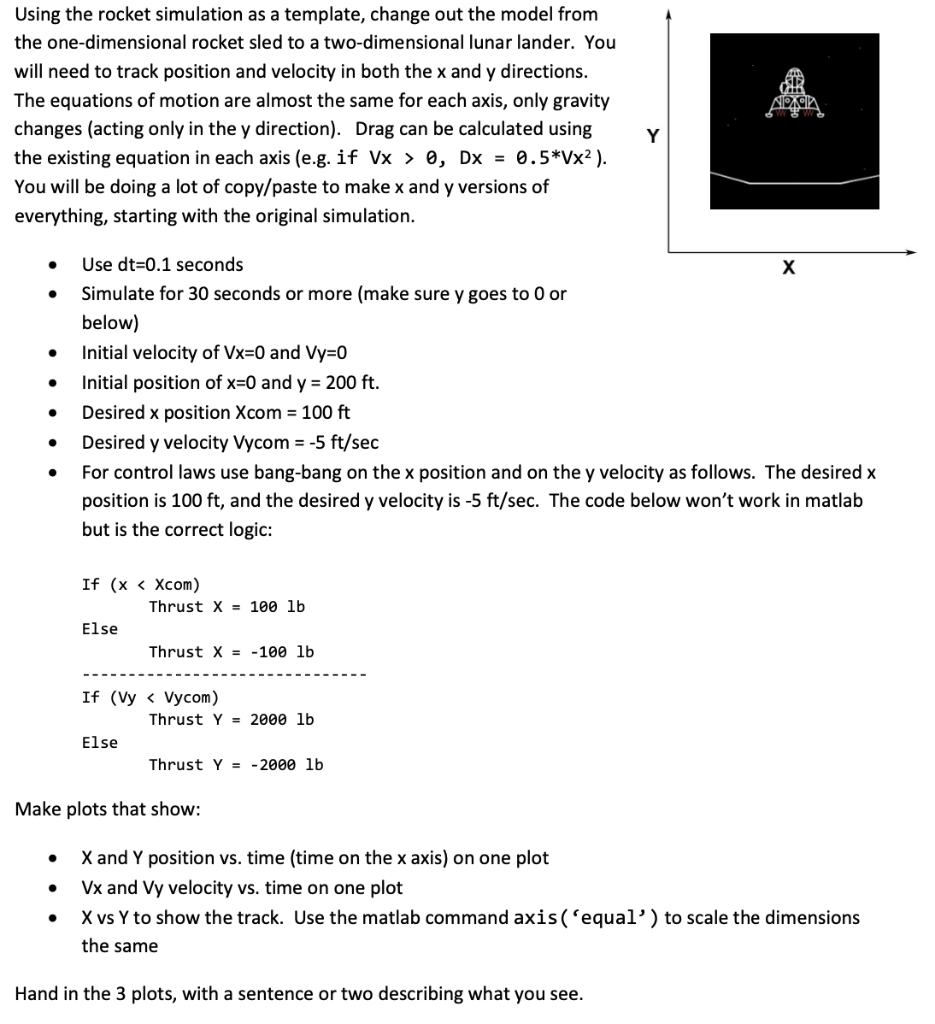
Using the rocket simulation as a template, change out the model from the one-dimensional rocket sled to a two-dimensional lunar lander. You will need to track position and velocity in both the x and y directions. The equations of motion are almost the same for each axis, only gravity changes (acting only in the y direction). Drag can be calculated using the existing equation in each axis (e.g. if Vx>0,Dx=0.5V2 ). You will be doing a lot of copy/paste to make x and y versions of everything, starting with the original simulation. - Use dt=0.1 seconds - Simulate for 30 seconds or more (make sure y goes to 0 or below) - Initial velocity of Vx=0 and Vy=0 - Initial position of x=0 and y=200ft. - Desired x position Xcom=100ft - Desired y velocity Vycom =5ft/sec - For control laws use bang-bang on the x position and on the y velocity as follows. The desired x position is 100ft, and the desired y velocity is 5ft/sec. The code below won't work in matlab but is the correct logic: Make plots that show: - X and Y position vs. time (time on the x axis) on one plot - Vx and Vy velocity vs. time on one plot - X vs Y to show the track. Use the matlab command axis ( 'equal') to scale the dimensions the same Hand in the 3 plots, with a sentence or two describing what you see. Using the rocket simulation as a template, change out the model from the one-dimensional rocket sled to a two-dimensional lunar lander. You will need to track position and velocity in both the x and y directions. The equations of motion are almost the same for each axis, only gravity changes (acting only in the y direction). Drag can be calculated using the existing equation in each axis (e.g. if Vx>0,Dx=0.5V2 ). You will be doing a lot of copy/paste to make x and y versions of everything, starting with the original simulation. - Use dt=0.1 seconds - Simulate for 30 seconds or more (make sure y goes to 0 or below) - Initial velocity of Vx=0 and Vy=0 - Initial position of x=0 and y=200ft. - Desired x position Xcom=100ft - Desired y velocity Vycom =5ft/sec - For control laws use bang-bang on the x position and on the y velocity as follows. The desired x position is 100ft, and the desired y velocity is 5ft/sec. The code below won't work in matlab but is the correct logic: Make plots that show: - X and Y position vs. time (time on the x axis) on one plot - Vx and Vy velocity vs. time on one plot - X vs Y to show the track. Use the matlab command axis ( 'equal') to scale the dimensions the same Hand in the 3 plots, with a sentence or two describing what you see