This is a question in Python.

I'm looking for help with part 4. This is the code I have but it doesn't seem to be working.

import numpy as np

import matplotlib.pyplot as plt

def solve_pendulum(FD, tend, type):

# Define parameters

q = 0.5

l = 9.8

g = 9.8

OmD = 2/3

dt = 0.04

tend = 100

theta0 = 0.2

omega0 = 0

# Define function for calculating the driving force

def F_drive(t, FD):

return FD*np.sin(OmD*t)

# Define function for calculating the total energy of the system

def E(theta, omega):

return 0.5*l**2*omega**2 + g*l*(1-np.cos(theta))

# Initialize arrays nsteps = int(tend/dt) t = np.zeros(nsteps) theta = np.zeros(nsteps) omega = np.zeros(nsteps) E_total = np.zeros(nsteps) # Set initial conditions theta[0] = theta0 omega[0] = omega0 # Calculate theta(t), omega(t), and E(t) using the Verlet method if type == 0: for i in range(1, nsteps): # Update position theta[i] = theta[i-1] + omega[i-1]*dt + 0.5*q*np.sin(theta[i-1])*dt**2\ + F_drive(i*dt, FD)*dt**2 # Update velocity omega[i] = omega[i-1] + 0.5*dt*(q*np.sin(theta[i]) + q*np.sin(theta[i-1]) \ - g/l*theta[i-1]) + F_drive(i*dt, FD)*dt # Update energy E_total[i] = E(theta[i], omega[i]) # Update time t[i] = i*dt print(F_drive(i*dt, FD)) # Plot Results plt.figure(figsize=(12, 6)) plt.subplot(2, 1, 1) plt.plot(t, theta) plt.xlabel('Time (s)') plt.ylabel('Angle (rad)') plt.title('Angle vs. Time, FD = {:.1f}'.format(FD)) plt.subplot(2, 1, 2) plt.plot(t, E_total) plt.xlabel('Time (s)') plt.ylabel('Total Energy (J)') plt.title('Total Energy vs. Time, FD = {:.1f}'.format(FD)) plt.tight_layout() plt.show() if FD == 0.5 or 1.2: return(theta, omega)

if type == 1: for i in range(1, nsteps): t[i] = i*dt if t[i] // (2 * np.pi / OmD) == 0: # Update position theta[i] = theta[i-1] + omega[i-1]*dt + 0.5*q*np.sin(theta[i-1])*dt**2\ + F_drive(i*dt, FD)*dt**2 # Update velocity omega[i] = omega[i-1] + 0.5*dt*(q*np.sin(theta[i]) + q*np.sin(theta[i-1]) \ - g/l*theta[i-1]) + F_drive(i*dt, FD)*dt # Update energy E_total[i] = E(theta[i], omega[i]) else: theta[i] = theta[i-1] omega[i] = omega[i-1] E_total[i] = E(theta[i], omega[i]) return(theta, omega) if type == 2: for i in range(1, nsteps): t[i] = i*dt if F_drive((i-1)*dt, FD) F_drive((i+1)*dt, FD): # Update position theta[i] = theta[i-1] + omega[i-1]*dt + 0.5*q*np.sin(theta[i-1])*dt**2\ + F_drive(i*dt, FD)*dt**2 # Update velocity omega[i] = omega[i-1] + 0.5*dt*(q*np.sin(theta[i]) + q*np.sin(theta[i-1]) \ - g/l*theta[i-1]) + F_drive(i*dt, FD)*dt # Update energy E_total[i] = E(theta[i], omega[i]) else: theta[i] = theta[i-1] omega[i] = omega[i-1] E_total[i] = E(theta[i], omega[i]) return(theta, omega)

# Part 2 solve_pendulum(0.1, 100, 0) theta05, omega05 = solve_pendulum(0.5, 100, 0) theta12, omega12 = solve_pendulum(1.2, 100, 0) # Part 3 plt.plot(theta05, omega05, label='FD = 0.5') plt.plot(theta12, omega12, label='FD = 1.2') plt.xlabel('Angle (rad)') plt.ylabel('Angular Velocity (rad/s)') plt.title('Angular Velocity vs. Angle') plt.legend() plt.show() # Part 4 theta5, omega5 = solve_pendulum(0.5, 10000, 1) theta2, omega2 = solve_pendulum(1.2, 10000, 1) plt.plot(theta5, omega5, label='FD = 0.5', ls = ':') plt.plot(theta2, omega2, label='FD = 1.2', ls = ':') plt.xlabel('Angle (rad)') plt.ylabel('Angular Velocity (rad/s)') plt.title('Poincare Section w/ t_end = 10000') plt.legend() plt.show()

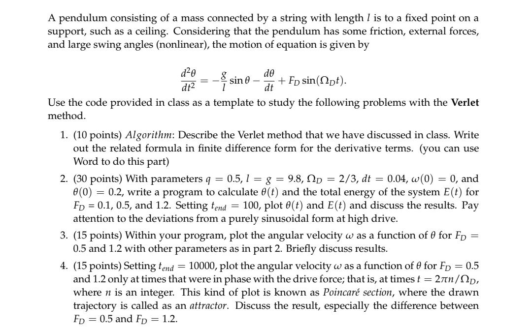
A pendulum consisting of a mass connected by a string with length l is to a fixed point on a support, such as a ceiling. Considering that the pendulum has some friction, external forces, and large swing angles (nonlinear), the motion of equation is given by dt2d2=lgsindtd+FDsin(Dt) Use the code provided in class as a template to study the following problems with the Verlet method. 1. (10 points) Algorithm: Describe the Verlet method that we have discussed in class. Write out the related formula in finite difference form for the derivative terms. (you can use Word to do this part) 2. (30 points) With parameters q=0.5,l=g=9.8,D=2/3,dt=0.04,(0)=0, and (0)=0.2, write a program to calculate (t) and the total energy of the system E(t) for FD=0.1,0.5, and 1.2. Setting tend=100, plot (t) and E(t) and discuss the results. Pay attention to the deviations from a purely sinusoidal form at high drive. 3. (15 points) Within your program, plot the angular velocity as a function of for FD= 0.5 and 1.2 with other parameters as in part 2 . Briefly discuss results. 4. (15 points) Setting tend=10000, plot the angular velocity as a function of for FD=0.5 and 1.2 only at times that were in phase with the drive force; that is, at times t=2n/D, where n is an integer. This kind of plot is known as Poincar section, where the drawn trajectory is called as an attractor. Discuss the result, especially the difference between FD=0.5 and FD=1.2