this is for my business data analytics class it is due tmr at 8am sharp! please help me submit this! this must be answered on excel sheet! thank you

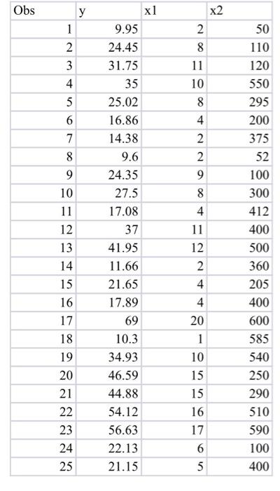
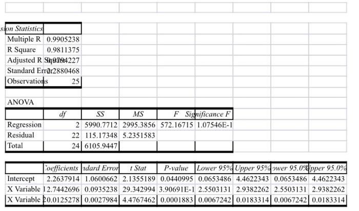
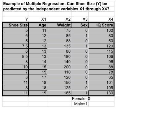
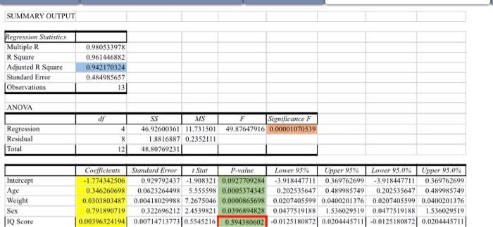
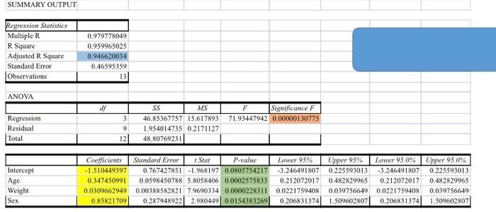
Obs x1 1 2 3 4 3 5 6 7 8 2 9 10 11 12 13 14 15 16 9.95 24.45 31.75 35 25.02 16.86 14.38 9.6 24.35 27.5 17.08 37 41.95 11.66 21.65 17.89 69 10.3 34.93 46.59 44.88 54.12 56.63 22.13 21.15 x2 2 8 11 10 8 4 2 2 9 8 4 11 12 2 4 4 20 1 10 15 15 16 17 6 50 110 120 550 295 200 375 52 100 300 412 400 500 360 205 400 600 585 540 250 290 510 590 100 400 17 18 19 20 21 22 23 24 25 sion Statistics Multiple R 0.9905238 R Square 0.9811375 Adjusted RS40784227 Standard Err@r2880468 Observations 25 ANOVA Regression Residual Total df SS MS F Significance F 2 5990.7712 2995.3856 572.16715 1.07546E-1 22 115.17348 5.2351583 24 6105.9447 oefficients ndard Error 1 Stat P-value Lower 95Upper 95% pwer 95.0"pper 95.0% Intercept 2.2637914 1.0600662 2.1355189 0.0440995 0.0653486 4.4622343 0.0653486 4.4622343 X Variable 12.7442696 0.0935238 29.342994 3.90691E-1 2.5503131 2.9382262 2.5503131 2.9382262 X Variable 20.0125278 0.0027984 4.4767462 0.0001883 0.0067242 0.0183314 0.0067242 0.0183314 Example of Multiple Regression: Can Shoe Size (Y) be predicted by the independent variables X1 through X4? 8 Y Shoe Size 5 6 5 7.5 6 8.5 8 10 7 8 11 8 11 X1 Age 11 12 12 13 13 13 14 15 15 17 18 18 19 X2 X3 Weight Sex 75 0 85 1 88 0 135 1 80 0 180 0 140 0 200 0 110 0 120 0 150 1 125 0 165 Female=0 Male=1 X4 IQ Score 100 80 50 120 115 106 96 88 78 65 101 105 130 8 SUMMARY OUTPUT Regression Statistics Multiple R R Square Adjusted R Square Standard Error Observations 0.980533978 0.961446882 0942170324 0.484985657 13 ANOVA dl Significance F 49.87647916 0.00001070539 Regression Residual Total 4 8 12 SS MS 46.92600361 11.731501 1.8816887 0.2352111 48.80769231 Intercept Age Weight Sex IQ Score Coefficients Standard Error + Star P-value Lower 95% Upper 95% Lower 95.0% Upper 95.0% -1.774342506 0.929792437 -1.908321 0.0927709284 -3.918447711 0.369762699 -3.918447711 0.369762699 0.346260698 0,0623264498 5.555598 0.0005374345 0.202535647 0.489985749 0.202535647 0.489985749 0.0303803487 0,00418029988 7.2675046 0.0000865698 0.0207405599 0.0400201376 0.0207405599 0.0400201376 0.791890719 0.322696212 2.4539821 0.0396894828 0.0477519188 1.536029519 0.0477519188 1.536029519 0.00396324194 0.007147137730.5545216 0.594380602 -0.0125180872 0.0204445711 -0.0125180872 0.0204445711 SUMMARY OUTPUT Regression Statistics Multiple R R Square Adjusted R Square Standard Error Observations 0.979778049 0.959965025 0.946620034 0.46595359 13 ANOVA d/ Significance F 71.93447942 0.00000130775 Regression Residual Total 3 9 12 SS MS 46.85367757 15.617893 1.954014735 0.2171127 48.80769231 Intercept Age Weight Sex Coefficients Standard Error Star P-wwe Lower 959 Upper 95% -1.510449397 0.767427851 -1.968197 0.0805754217 -3.246491807 0.225593013 0.347450991 0.0598450788 5.8058406 0.0002575833 0.212072017 0.482829965 0.0309662949 0.00388582821 7.9690334 0.0000228311 0.0221759408 0.039756649 0.85821709 0.287948922 2.980449 0.0154383269 0.206831374 1.509602807 Lower 95.0% Une 95.0% -3.246491807 0.225593013 0.212072012 0.482829965 0,0221759408 0.039756649 0.2068313741 1.509602807 Obs x1 1 2 3 4 3 5 6 7 8 2 9 10 11 12 13 14 15 16 9.95 24.45 31.75 35 25.02 16.86 14.38 9.6 24.35 27.5 17.08 37 41.95 11.66 21.65 17.89 69 10.3 34.93 46.59 44.88 54.12 56.63 22.13 21.15 x2 2 8 11 10 8 4 2 2 9 8 4 11 12 2 4 4 20 1 10 15 15 16 17 6 50 110 120 550 295 200 375 52 100 300 412 400 500 360 205 400 600 585 540 250 290 510 590 100 400 17 18 19 20 21 22 23 24 25 sion Statistics Multiple R 0.9905238 R Square 0.9811375 Adjusted RS40784227 Standard Err@r2880468 Observations 25 ANOVA Regression Residual Total df SS MS F Significance F 2 5990.7712 2995.3856 572.16715 1.07546E-1 22 115.17348 5.2351583 24 6105.9447 oefficients ndard Error 1 Stat P-value Lower 95Upper 95% pwer 95.0"pper 95.0% Intercept 2.2637914 1.0600662 2.1355189 0.0440995 0.0653486 4.4622343 0.0653486 4.4622343 X Variable 12.7442696 0.0935238 29.342994 3.90691E-1 2.5503131 2.9382262 2.5503131 2.9382262 X Variable 20.0125278 0.0027984 4.4767462 0.0001883 0.0067242 0.0183314 0.0067242 0.0183314 Example of Multiple Regression: Can Shoe Size (Y) be predicted by the independent variables X1 through X4? 8 Y Shoe Size 5 6 5 7.5 6 8.5 8 10 7 8 11 8 11 X1 Age 11 12 12 13 13 13 14 15 15 17 18 18 19 X2 X3 Weight Sex 75 0 85 1 88 0 135 1 80 0 180 0 140 0 200 0 110 0 120 0 150 1 125 0 165 Female=0 Male=1 X4 IQ Score 100 80 50 120 115 106 96 88 78 65 101 105 130 8 SUMMARY OUTPUT Regression Statistics Multiple R R Square Adjusted R Square Standard Error Observations 0.980533978 0.961446882 0942170324 0.484985657 13 ANOVA dl Significance F 49.87647916 0.00001070539 Regression Residual Total 4 8 12 SS MS 46.92600361 11.731501 1.8816887 0.2352111 48.80769231 Intercept Age Weight Sex IQ Score Coefficients Standard Error + Star P-value Lower 95% Upper 95% Lower 95.0% Upper 95.0% -1.774342506 0.929792437 -1.908321 0.0927709284 -3.918447711 0.369762699 -3.918447711 0.369762699 0.346260698 0,0623264498 5.555598 0.0005374345 0.202535647 0.489985749 0.202535647 0.489985749 0.0303803487 0,00418029988 7.2675046 0.0000865698 0.0207405599 0.0400201376 0.0207405599 0.0400201376 0.791890719 0.322696212 2.4539821 0.0396894828 0.0477519188 1.536029519 0.0477519188 1.536029519 0.00396324194 0.007147137730.5545216 0.594380602 -0.0125180872 0.0204445711 -0.0125180872 0.0204445711 SUMMARY OUTPUT Regression Statistics Multiple R R Square Adjusted R Square Standard Error Observations 0.979778049 0.959965025 0.946620034 0.46595359 13 ANOVA d/ Significance F 71.93447942 0.00000130775 Regression Residual Total 3 9 12 SS MS 46.85367757 15.617893 1.954014735 0.2171127 48.80769231 Intercept Age Weight Sex Coefficients Standard Error Star P-wwe Lower 959 Upper 95% -1.510449397 0.767427851 -1.968197 0.0805754217 -3.246491807 0.225593013 0.347450991 0.0598450788 5.8058406 0.0002575833 0.212072017 0.482829965 0.0309662949 0.00388582821 7.9690334 0.0000228311 0.0221759408 0.039756649 0.85821709 0.287948922 2.980449 0.0154383269 0.206831374 1.509602807 Lower 95.0% Une 95.0% -3.246491807 0.225593013 0.212072012 0.482829965 0,0221759408 0.039756649 0.2068313741 1.509602807