this is for my Data Analysis class, would you help me with (6.1, 6.2, 6.3, 6.6, 6.10)

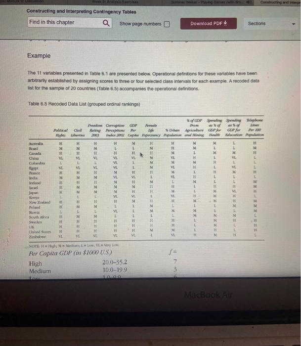
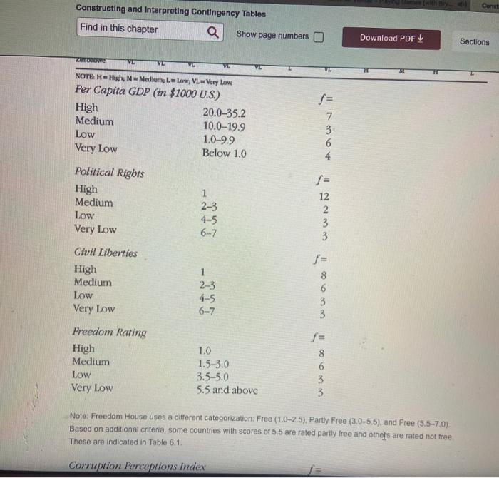
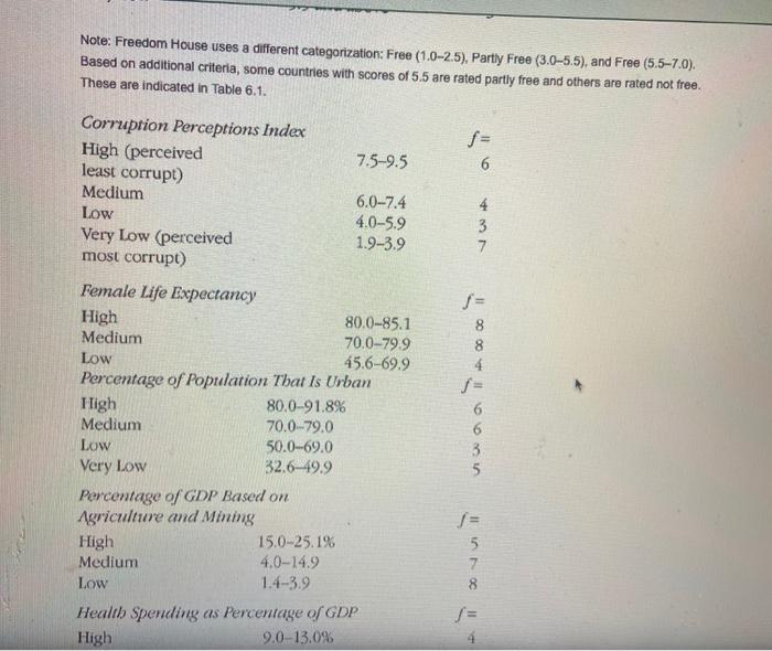
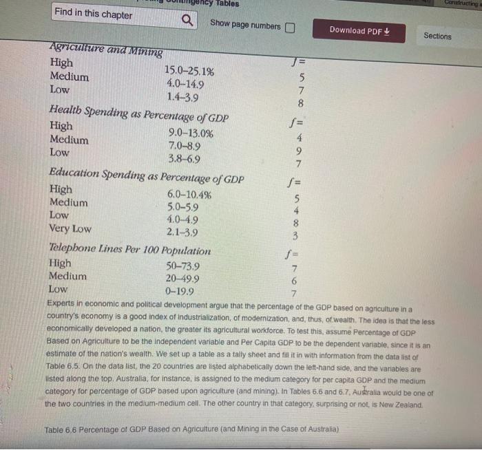
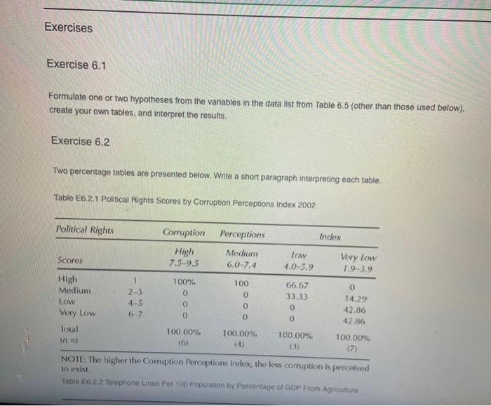
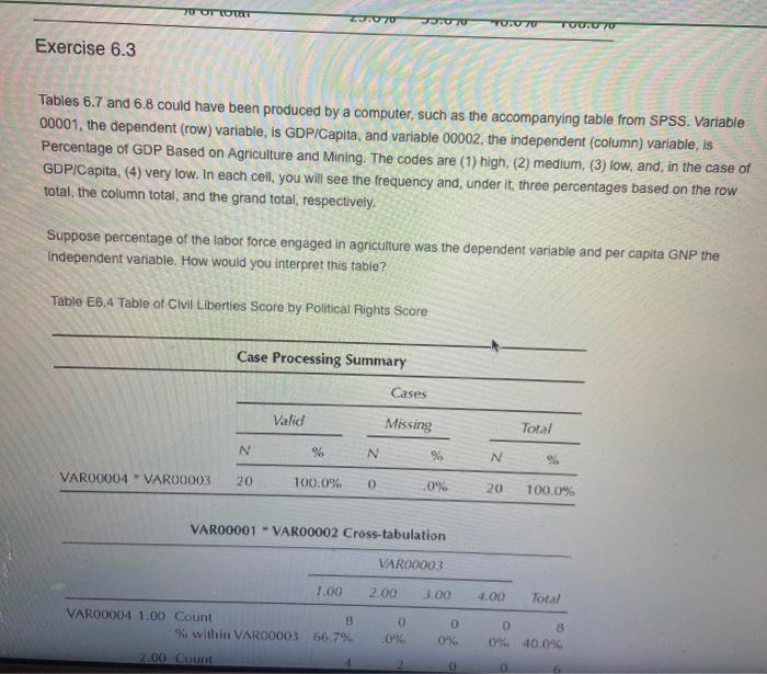
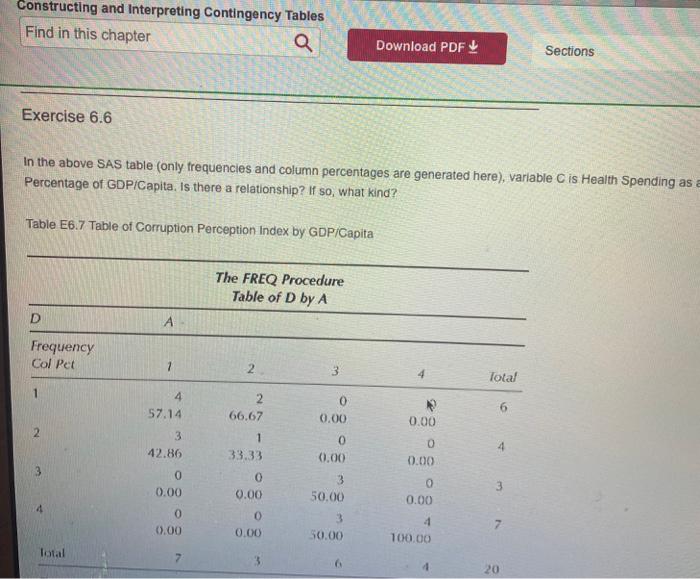
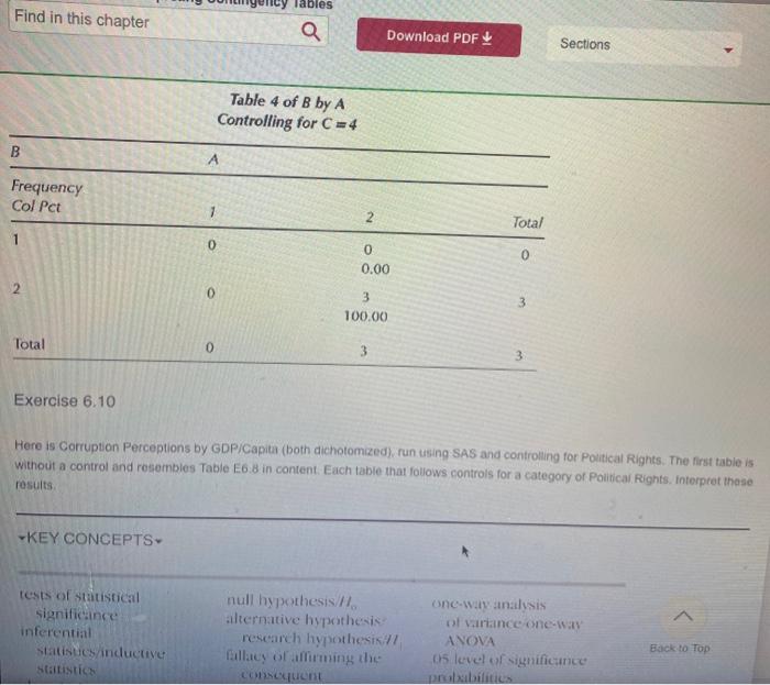
Constructing and Interpreting Contingency Tables Find in this chapter Q Show page numbers Download PDF Sections Example The 11 variables presented in Table 6.1 are presented below. Operational definitions for these variables have been arbitrarily established by assigning scores to three or four selected class intervals for each example. A recoded data list for the sample of 20 countries (Table 6.5) accompanies the operational definitions. Table 6.5 Recoded Data List (grouped ordinal rankings) Paul Gu Australia H M IL VE Canada Columbia Mence India Ireland Israe J VE H M 11 L VE H M H M M SGP Spiderman Freedom Corruption GDP Female as More her Urban Agricul GOP for GDP for 2003 Sai pala y Agalaium Mirai Titals April H M M L 1 M 11 M M 11 H M M M 11 VL M VL H L VL 1 M H VL M VE VE H M M 1 M H M VL VL L H M 1 M L L N M H 11 M H M VI. H VE 1 VE M H M 1 M t VL M N N 11 11 H H N H M V VE H mmutum = "m"htm SZESZESSE SESEZE SES=2 H M New and Poland Sam South Aina Sweden UK --- M H H H H VE XX Zimbabwe /= SOTE HHud Mumt. Vym Per Capita GDP (in $1000 U.S) High 20.0-35.2 Medium 10.0-19.9 La 100 MacBook Air Const Constructing and Interpreting Contingency Tables Find in this chapter Q Show page numbers o Download PDF Sections ZIONE VL VE VO VL VL NOTE High: Medium Low; VL Very low Per Capita GDP (in $1000 U.S.) High 20.0-35.2 Medium 10.0-19.9 Low 1.0-9.9 Very Low Below 1.0 = 7 3 6 4 Political Rights High Medium Low Very Low 2-3 4-5 6-7 12 2 3 3 Civil Liberties High Medium Low Very Low 1 2-3 4-5 6-7 f= 8 6 3 3 Freedom Rating High Medium Low 1.0 1.5 3.0 3.5-5.0 5.5 and above 8 6 3 3 Very Low Note: Freedom House uses a different categorization: Free (1.0-2.5). Partly Free (3.0-5,5), and Free (5.5-7.0). Based on additional criteria, some countries with scores of 5,5 are rated partly free and othe's are rated not free These are indicated in Table 6.1. Corruption Perceptions Index Note: Freedom House uses a different categorization: Free (1.0-2.5), Partly Free (3.0-5.5), and Free (5.5-7.0). Based on additional criteria, some countries with scores of 5.5 are rated partly free and others are rated not free. These are indicated in Table 6.1. f= 6 4 3 7 8 Corruption Perceptions Index High (perceived 7.5-9.5 least corrupt) Medium 6.0-7.4 Low 4.0-5.9 Very Low (perceived 1.9-3.9 most corrupt) Female Life Expectancy High 80.0-85.1 Medium 70.0-79.9 Low 45.6-69.9 Percentage of Population That Is Urban High 80.0-91.8% Medium 70.0-79.0 Low 50.0-69.0 Very Low 32.6-49.9 Percentage of GDP Based on Agriculture and Mining High 15.0-25.196 Medium 4.0-14.9 Low 1.4-3.9 Health Spending as Percentage of GDP High 9.0-13.0% 6 3 5 5 7 8 J = + ncy Tables Find in this chapter a Show page numbers o Download PDF Sections A Agriculture and Mining JE High 15.0-25.1% Medium 5 4.0-14.9 Low 7 1.4-3.9 8 Health Spending as Percentage of GDP High 9.0-13.0% 4 Medium 7.0-8.9 9 Low 3.8-6.9 7 Education Spending as Percentage of GDP S = High 6.0-10.4% 5 Medium 5.0-5.9 Low 4.0-4.9 Very Low 2.1-3.9 3 Telepbone Lines Per 100 Population High 50-73.9 7 Medium 20-49.9 6 Low 0-19.9 7 Experts in economic and political development argue that the percentage of the GDP based on agriculture in a country's economy is a good index of industrialization of modernization, and thus of wealth. The idea is that the less economically developed a nation, the greater its agricultural workforce. To test this, assume Percentage of GDP Based on Agriculture to be the Independent variable and Per Capita GDP to be the dependent variable, since it is an estimate of the nation's wealth. We set up a table as a tally sheet and fill it in with information from the data list of Table 6.5. On the data list, the 20 countries are listed alphabetically down the left-hand side, and the variables are listed along the top. Australia, for instance, is assigned to the medium category for per capita GDP and the medium category for percentage of GDP based upon agriculture and mining). In Tables 6.6 and 6.7. Australia would be one of the two countries in the medium-medium cell. The other country in that category, surprising or not, is New Zealand. Table 6.6 Percentage of GDP Based on Agriculture (and Mining in the case of Australia) Exercises Exercise 6.1 Formulate one or two hypotheses from the variables in the data list from Table 6.5 (other than those used below), create your own tables, and interpret the results, Exercise 6.2 Two percentage tables are presented below. Write a short paragraph Interpreting each table. Table E6.2.1 Political Rights Scores by Corruption Perceptions Index 2002 Political Rights Corruption Perceptions Index Scores High 7.5-9.5 Medium 6,0-7.4 Low 4.0-5.9 Very low 1.9-3.9 High Medium LOW Very Low Total 1 2-3 4-5 67 100% 0 0 66.67 33.33 100 0 0 0 0 14.29 42.86 42.86 0 100.00% (6) 100.00% 100.00% 100.00% NOTE: The higher the Corruption Perceptions Index, the less corruption is perceived to exist Table E6 2.2 Telephone Linos Per 100 Population by Parcentage of GDP From Agriculture Constructing and Interpreting Contingency Tables Find in this chapter Q Show page numbers o Download PDF NOTE: The higher the Corruption Perceptions Index, the less corruption is perceived to exist. Table E6.2.2 Telephone Lines Per 100 Population by Percentage of GDP From Agriculture Percentage of GDP From Agriculture High Medium Low 15.0 25.1% 4.0 14.9% 1.4-3.9% Telephone Lines Per 100 Population High Medium Low 50-73.9 20-49.9 0-19.9 0% 0 100.0 14.3 57.1 28.6 75.0 25.0 Total in =) 100.0% (5) 100.0% (7) 100.0% (8) Table E6.3 Table of GDP/Capita by Percentage of GDP From Agriculture Crosstabs Case Processing Summary Cases Valid Missing Total N N N VAR00001" VARO0002 %6 20 100.0% O 20 100.0% VAR00001 - VARO0002 Cross-tabulation VAROO Constructing and Interpreting Contingency Tables Find in this chapter Show page numbers Download PDF VAR00001 *VARO0002 Cross-tabulation VARO0002 7.00 2.00 3.00 Total VARO0001 1.00 Count % within VAR00001 % within VAR00002 % of total 0 -0% .0% 1 14.3% 14.3% 5.0% 6 85.7% 75.0% 30.0% 7 100.0% 35.0% 35.0% 0% 2.00 Count % within VARO0001 % within VARO0002 % of total 0 .0% 0% .0% 2 66.7% 28.6% 10.0% 1 33.3% 12.5% 5.0% 3 100.0% 15.0% 15.0% 3.00 Count % within VARO0001 % within VAR00002 % of total 1 16.796 20.0% 5.0% 4 66.7% 57.1% 20.0% 1 16.7% 12.5% 5.0% 100.0% 30.0% 30.0% 4.00 Count % within VAR00001 % within VAR00002 % of total 4 100.0% 80.0% 20.0% 0 0% ,0% o 0% .0% -0% 4 100.0% 20.0% 20.0% .0% Total Count 5 7 8 % within VARO0001 25.0% 35.0% 40.0 % within VARO0002 100.0% 100.0% 100.0% % of total 25.0% 35.0% 40.0% 20 100.0% 100.0% 100.0% Exercise 6.3 70 UT KOMT 2070 JUU TURUT Exercise 6.3 Tables 6.7 and 6.8 could have been produced by a computer, such as the accompanying table from SPSS. Variable 00001, the dependent (row) variable, is GDP/Capita, and variable 00002, the independent (column) variable, is Percentage of GDP Based on Agriculture and Mining. The codes are (1) high, (2) medium, (3) low, and in the case of GDP/Capita, (4) very low. In each cell, you will see the frequency and, under it, three percentages based on the row total, the column total, and the grand total, respectively. Suppose percentage of the labor force engaged in agriculture was the dependent variable and per capita GNP the independent variable. How would you interpret this table? Table E6,4 Table of Civil Liberties Score by Political Rights Score Case Processing Summary Cases Valid Missing Total N % N % N VARO0004 VARO0003 20 100.0% 0 -0% 20 100.0% VARO0001 - VARO0002 Cross-tabulation VARO0003 1.00 2.00 3.00 4.00 Total VARO0004 1.00 Count % within VAR00003 66.7% 0 .0 0 OX 0 8 0% 40.09 Constructing and Interpreting Contingency Tables Find in this chapter Q Show page numbers o Download PDF VARO0001 VARO0002 Cross-tabulation VAR00003 1.00 2.00 3.00 4.00 Total VAR00004 1.00 Count 8 % within VARO0003 66.7% 0 .0% .0% 8 .0% 40.0% 2.00 Count 2 % within VAR00003 33.3% 100.0% 0 6 .0% 30.0% .0% 3.00 Count % within VAR00003 0 .0% 0 3 0% 100.0% 0 .0% 15.0% 0 4.00 Count % within VAR00003 0 .0% .0%. 0 3 .0% 100.0% 15.0% Total Count 12 2 3 3 20 % within VARO0003 100.0% 100.0% 100.0% 100.0% 100.0% Exercise 6.4 In the table above, a nation's Civil Liberties score is dependent on the independent variable Political Rights. Interpret the table. VAR00004 is the Civil Liberties score, and VAR00003 is the Political Rights score. Only the column percentages are reported here. Table E6.5.1 Table of Telephone Lines Per 100 Population by GOP/Capita Case Processing Summary Valid Missing Toad percentages are reported here. Table E6.5.1 Table of Telephone Lines Per 100 Population by GDP/Capita Case Processing Summary Cases Valid Missing Total N % N % N % VAR00005 * VARO0001 20 100.0% 0 .0% 20 100.0% VAR00005 * VAR00005 Cross-tabulation VAR00001 1.00 2.00 3.00 4.00 Total VARO0005 1.00 Count 6 1 % within VAR0000185.7% 33.3% 0 .0% 0 7 .0% 35.0% 2.00 Count 2 % within VARO0001 14.3% 66.7% 50.0% 0 6 .0% 30.0% 3.00 Count % within VAR00001 0 0% 3 4 7 .0% 50.0% 100.0% 35.0% Total Count 7 3 6 4 20 % within VARO0001 100.0% 100.0% 100.0% 100.0% 100.0% Exercise 6.5 Constructing and Interpreting Contingency Tables Find in this chapter a Download PDF Sections Exercise 6.6 In the above SAS table (only frequencies and column percentages are generated here), variable C is Health Spending as a Percentage of GDP/Capita. Is there a relationship? If so, what kind? Table E6.7 Table of Corruption Perception Index by GDP/Capita The FREQ Procedure Table of D by A D Frequency Col Pet 7 -2 3 4 Total 1 2 66.67 0 0.00 6 4 57.14 3 42.86 0.00 1 33.33 0 0.00 4 0 0.00 0 0.00 3 50.00 3 0 0.00 0 0.00 0 0.00 0 0.00 3 50.00 7 4 100.00 Total 20 Tables Find in this chapter Download PDF Sections Table 4 of B by A Controlling for C=4 B Frequency Col Pet 1 2 Total 1 0 0 0.00 0 2 0 3 100.00 3 Total 0 3 3 Exercise 6.10 Here is corruption Perceptions by GDP/Capita (both dichotomized), run using SAS and controlling for Political Rights. The first table is without a control and resembles Table E68 in content. Each table that follows controls for a category of Political Rights. Interpret those rosults -KEY CONCEPTS TOSIS Ol Statistical significance inferential Statistics inductive SLISTIC null hypothesis/ alternative hypothesis research hypothesis: fallacy olaffirming the Consequent One-way analysis of variance one-way ANOVA 05 level of significance Back to Top Constructing and Interpreting Contingency Tables Find in this chapter Q Show page numbers Download PDF Sections Example The 11 variables presented in Table 6.1 are presented below. Operational definitions for these variables have been arbitrarily established by assigning scores to three or four selected class intervals for each example. A recoded data list for the sample of 20 countries (Table 6.5) accompanies the operational definitions. Table 6.5 Recoded Data List (grouped ordinal rankings) Paul Gu Australia H M IL VE Canada Columbia Mence India Ireland Israe J VE H M 11 L VE H M H M M SGP Spiderman Freedom Corruption GDP Female as More her Urban Agricul GOP for GDP for 2003 Sai pala y Agalaium Mirai Titals April H M M L 1 M 11 M M 11 H M M M 11 VL M VL H L VL 1 M H VL M VE VE H M M 1 M H M VL VL L H M 1 M L L N M H 11 M H M VI. H VE 1 VE M H M 1 M t VL M N N 11 11 H H N H M V VE H mmutum = "m"htm SZESZESSE SESEZE SES=2 H M New and Poland Sam South Aina Sweden UK --- M H H H H VE XX Zimbabwe /= SOTE HHud Mumt. Vym Per Capita GDP (in $1000 U.S) High 20.0-35.2 Medium 10.0-19.9 La 100 MacBook Air Const Constructing and Interpreting Contingency Tables Find in this chapter Q Show page numbers o Download PDF Sections ZIONE VL VE VO VL VL NOTE High: Medium Low; VL Very low Per Capita GDP (in $1000 U.S.) High 20.0-35.2 Medium 10.0-19.9 Low 1.0-9.9 Very Low Below 1.0 = 7 3 6 4 Political Rights High Medium Low Very Low 2-3 4-5 6-7 12 2 3 3 Civil Liberties High Medium Low Very Low 1 2-3 4-5 6-7 f= 8 6 3 3 Freedom Rating High Medium Low 1.0 1.5 3.0 3.5-5.0 5.5 and above 8 6 3 3 Very Low Note: Freedom House uses a different categorization: Free (1.0-2.5). Partly Free (3.0-5,5), and Free (5.5-7.0). Based on additional criteria, some countries with scores of 5,5 are rated partly free and othe's are rated not free These are indicated in Table 6.1. Corruption Perceptions Index Note: Freedom House uses a different categorization: Free (1.0-2.5), Partly Free (3.0-5.5), and Free (5.5-7.0). Based on additional criteria, some countries with scores of 5.5 are rated partly free and others are rated not free. These are indicated in Table 6.1. f= 6 4 3 7 8 Corruption Perceptions Index High (perceived 7.5-9.5 least corrupt) Medium 6.0-7.4 Low 4.0-5.9 Very Low (perceived 1.9-3.9 most corrupt) Female Life Expectancy High 80.0-85.1 Medium 70.0-79.9 Low 45.6-69.9 Percentage of Population That Is Urban High 80.0-91.8% Medium 70.0-79.0 Low 50.0-69.0 Very Low 32.6-49.9 Percentage of GDP Based on Agriculture and Mining High 15.0-25.196 Medium 4.0-14.9 Low 1.4-3.9 Health Spending as Percentage of GDP High 9.0-13.0% 6 3 5 5 7 8 J = + ncy Tables Find in this chapter a Show page numbers o Download PDF Sections A Agriculture and Mining JE High 15.0-25.1% Medium 5 4.0-14.9 Low 7 1.4-3.9 8 Health Spending as Percentage of GDP High 9.0-13.0% 4 Medium 7.0-8.9 9 Low 3.8-6.9 7 Education Spending as Percentage of GDP S = High 6.0-10.4% 5 Medium 5.0-5.9 Low 4.0-4.9 Very Low 2.1-3.9 3 Telepbone Lines Per 100 Population High 50-73.9 7 Medium 20-49.9 6 Low 0-19.9 7 Experts in economic and political development argue that the percentage of the GDP based on agriculture in a country's economy is a good index of industrialization of modernization, and thus of wealth. The idea is that the less economically developed a nation, the greater its agricultural workforce. To test this, assume Percentage of GDP Based on Agriculture to be the Independent variable and Per Capita GDP to be the dependent variable, since it is an estimate of the nation's wealth. We set up a table as a tally sheet and fill it in with information from the data list of Table 6.5. On the data list, the 20 countries are listed alphabetically down the left-hand side, and the variables are listed along the top. Australia, for instance, is assigned to the medium category for per capita GDP and the medium category for percentage of GDP based upon agriculture and mining). In Tables 6.6 and 6.7. Australia would be one of the two countries in the medium-medium cell. The other country in that category, surprising or not, is New Zealand. Table 6.6 Percentage of GDP Based on Agriculture (and Mining in the case of Australia) Exercises Exercise 6.1 Formulate one or two hypotheses from the variables in the data list from Table 6.5 (other than those used below), create your own tables, and interpret the results, Exercise 6.2 Two percentage tables are presented below. Write a short paragraph Interpreting each table. Table E6.2.1 Political Rights Scores by Corruption Perceptions Index 2002 Political Rights Corruption Perceptions Index Scores High 7.5-9.5 Medium 6,0-7.4 Low 4.0-5.9 Very low 1.9-3.9 High Medium LOW Very Low Total 1 2-3 4-5 67 100% 0 0 66.67 33.33 100 0 0 0 0 14.29 42.86 42.86 0 100.00% (6) 100.00% 100.00% 100.00% NOTE: The higher the Corruption Perceptions Index, the less corruption is perceived to exist Table E6 2.2 Telephone Linos Per 100 Population by Parcentage of GDP From Agriculture Constructing and Interpreting Contingency Tables Find in this chapter Q Show page numbers o Download PDF NOTE: The higher the Corruption Perceptions Index, the less corruption is perceived to exist. Table E6.2.2 Telephone Lines Per 100 Population by Percentage of GDP From Agriculture Percentage of GDP From Agriculture High Medium Low 15.0 25.1% 4.0 14.9% 1.4-3.9% Telephone Lines Per 100 Population High Medium Low 50-73.9 20-49.9 0-19.9 0% 0 100.0 14.3 57.1 28.6 75.0 25.0 Total in =) 100.0% (5) 100.0% (7) 100.0% (8) Table E6.3 Table of GDP/Capita by Percentage of GDP From Agriculture Crosstabs Case Processing Summary Cases Valid Missing Total N N N VAR00001" VARO0002 %6 20 100.0% O 20 100.0% VAR00001 - VARO0002 Cross-tabulation VAROO Constructing and Interpreting Contingency Tables Find in this chapter Show page numbers Download PDF VAR00001 *VARO0002 Cross-tabulation VARO0002 7.00 2.00 3.00 Total VARO0001 1.00 Count % within VAR00001 % within VAR00002 % of total 0 -0% .0% 1 14.3% 14.3% 5.0% 6 85.7% 75.0% 30.0% 7 100.0% 35.0% 35.0% 0% 2.00 Count % within VARO0001 % within VARO0002 % of total 0 .0% 0% .0% 2 66.7% 28.6% 10.0% 1 33.3% 12.5% 5.0% 3 100.0% 15.0% 15.0% 3.00 Count % within VARO0001 % within VAR00002 % of total 1 16.796 20.0% 5.0% 4 66.7% 57.1% 20.0% 1 16.7% 12.5% 5.0% 100.0% 30.0% 30.0% 4.00 Count % within VAR00001 % within VAR00002 % of total 4 100.0% 80.0% 20.0% 0 0% ,0% o 0% .0% -0% 4 100.0% 20.0% 20.0% .0% Total Count 5 7 8 % within VARO0001 25.0% 35.0% 40.0 % within VARO0002 100.0% 100.0% 100.0% % of total 25.0% 35.0% 40.0% 20 100.0% 100.0% 100.0% Exercise 6.3 70 UT KOMT 2070 JUU TURUT Exercise 6.3 Tables 6.7 and 6.8 could have been produced by a computer, such as the accompanying table from SPSS. Variable 00001, the dependent (row) variable, is GDP/Capita, and variable 00002, the independent (column) variable, is Percentage of GDP Based on Agriculture and Mining. The codes are (1) high, (2) medium, (3) low, and in the case of GDP/Capita, (4) very low. In each cell, you will see the frequency and, under it, three percentages based on the row total, the column total, and the grand total, respectively. Suppose percentage of the labor force engaged in agriculture was the dependent variable and per capita GNP the independent variable. How would you interpret this table? Table E6,4 Table of Civil Liberties Score by Political Rights Score Case Processing Summary Cases Valid Missing Total N % N % N VARO0004 VARO0003 20 100.0% 0 -0% 20 100.0% VARO0001 - VARO0002 Cross-tabulation VARO0003 1.00 2.00 3.00 4.00 Total VARO0004 1.00 Count % within VAR00003 66.7% 0 .0 0 OX 0 8 0% 40.09 Constructing and Interpreting Contingency Tables Find in this chapter Q Show page numbers o Download PDF VARO0001 VARO0002 Cross-tabulation VAR00003 1.00 2.00 3.00 4.00 Total VAR00004 1.00 Count 8 % within VARO0003 66.7% 0 .0% .0% 8 .0% 40.0% 2.00 Count 2 % within VAR00003 33.3% 100.0% 0 6 .0% 30.0% .0% 3.00 Count % within VAR00003 0 .0% 0 3 0% 100.0% 0 .0% 15.0% 0 4.00 Count % within VAR00003 0 .0% .0%. 0 3 .0% 100.0% 15.0% Total Count 12 2 3 3 20 % within VARO0003 100.0% 100.0% 100.0% 100.0% 100.0% Exercise 6.4 In the table above, a nation's Civil Liberties score is dependent on the independent variable Political Rights. Interpret the table. VAR00004 is the Civil Liberties score, and VAR00003 is the Political Rights score. Only the column percentages are reported here. Table E6.5.1 Table of Telephone Lines Per 100 Population by GOP/Capita Case Processing Summary Valid Missing Toad percentages are reported here. Table E6.5.1 Table of Telephone Lines Per 100 Population by GDP/Capita Case Processing Summary Cases Valid Missing Total N % N % N % VAR00005 * VARO0001 20 100.0% 0 .0% 20 100.0% VAR00005 * VAR00005 Cross-tabulation VAR00001 1.00 2.00 3.00 4.00 Total VARO0005 1.00 Count 6 1 % within VAR0000185.7% 33.3% 0 .0% 0 7 .0% 35.0% 2.00 Count 2 % within VARO0001 14.3% 66.7% 50.0% 0 6 .0% 30.0% 3.00 Count % within VAR00001 0 0% 3 4 7 .0% 50.0% 100.0% 35.0% Total Count 7 3 6 4 20 % within VARO0001 100.0% 100.0% 100.0% 100.0% 100.0% Exercise 6.5 Constructing and Interpreting Contingency Tables Find in this chapter a Download PDF Sections Exercise 6.6 In the above SAS table (only frequencies and column percentages are generated here), variable C is Health Spending as a Percentage of GDP/Capita. Is there a relationship? If so, what kind? Table E6.7 Table of Corruption Perception Index by GDP/Capita The FREQ Procedure Table of D by A D Frequency Col Pet 7 -2 3 4 Total 1 2 66.67 0 0.00 6 4 57.14 3 42.86 0.00 1 33.33 0 0.00 4 0 0.00 0 0.00 3 50.00 3 0 0.00 0 0.00 0 0.00 0 0.00 3 50.00 7 4 100.00 Total 20 Tables Find in this chapter Download PDF Sections Table 4 of B by A Controlling for C=4 B Frequency Col Pet 1 2 Total 1 0 0 0.00 0 2 0 3 100.00 3 Total 0 3 3 Exercise 6.10 Here is corruption Perceptions by GDP/Capita (both dichotomized), run using SAS and controlling for Political Rights. The first table is without a control and resembles Table E68 in content. Each table that follows controls for a category of Political Rights. Interpret those rosults -KEY CONCEPTS TOSIS Ol Statistical significance inferential Statistics inductive SLISTIC null hypothesis/ alternative hypothesis research hypothesis: fallacy olaffirming the Consequent One-way analysis of variance one-way ANOVA 05 level of significance Back to Top