This is statistics course, sampling distributions, estimation and tests of significance units.I need help with this. I attached formula sheet in case you need it.

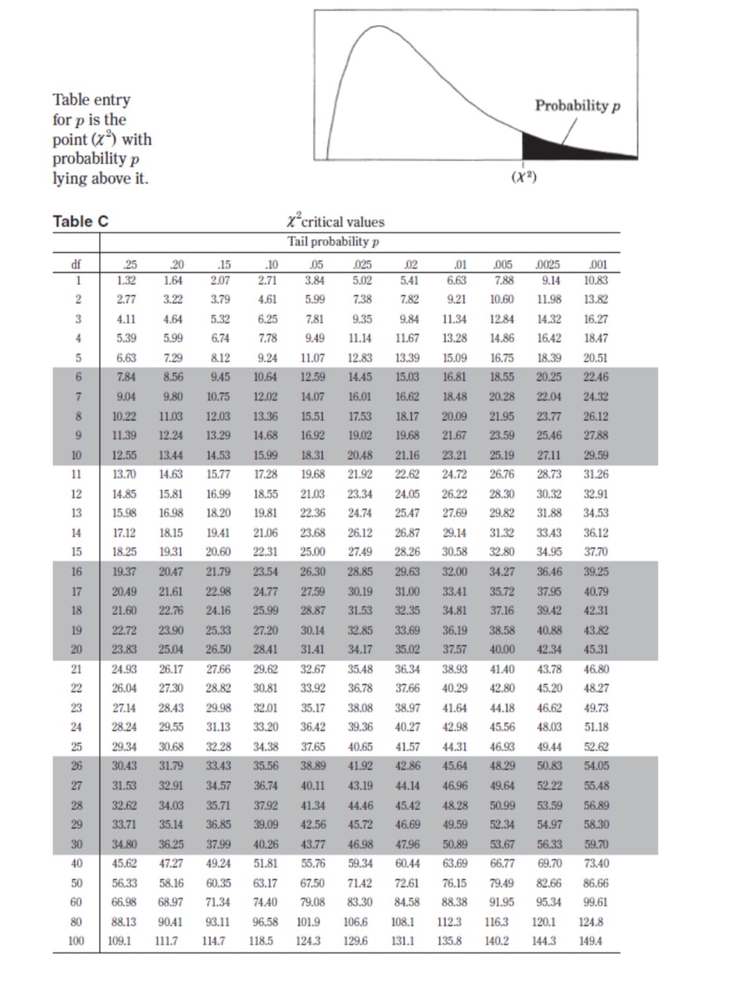
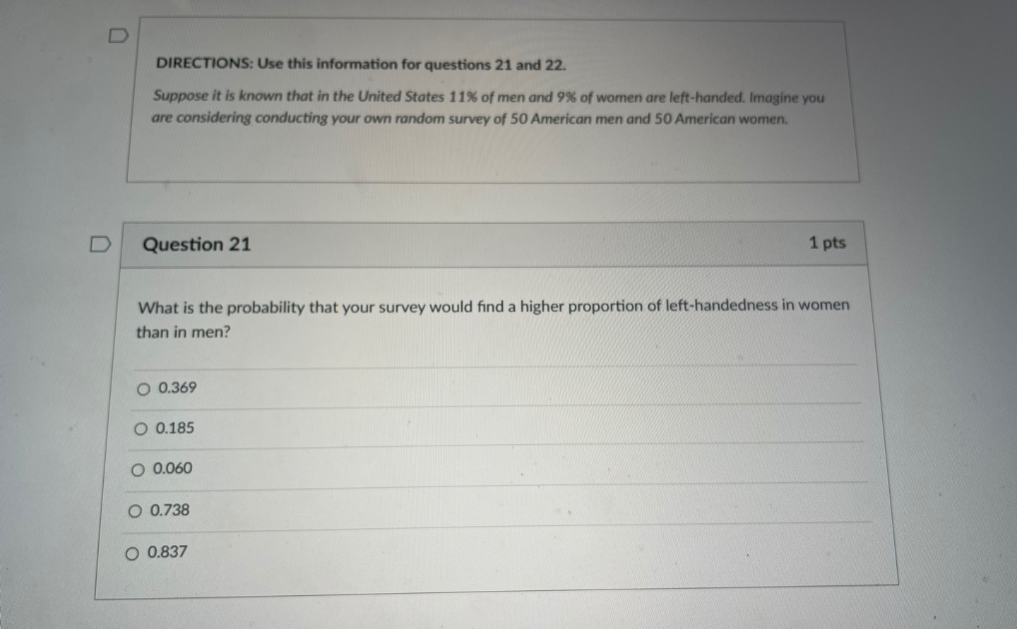
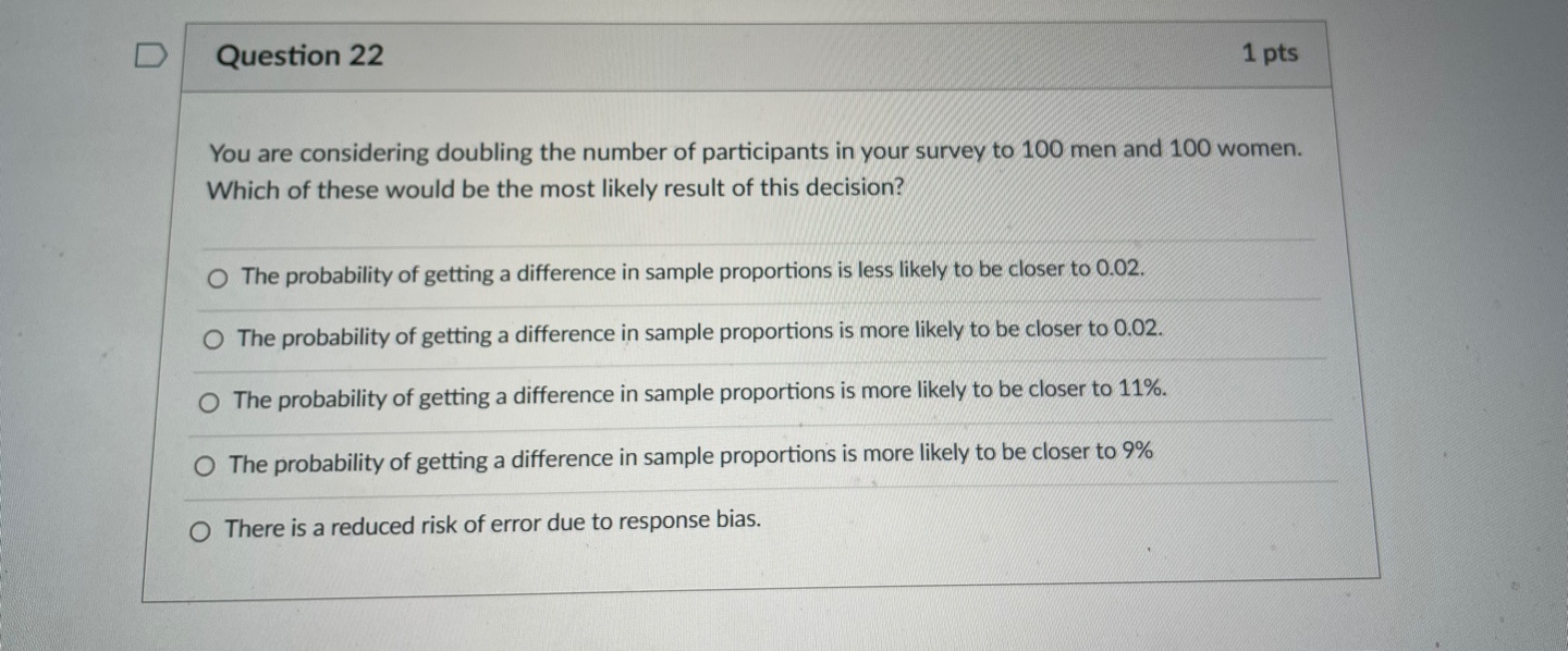
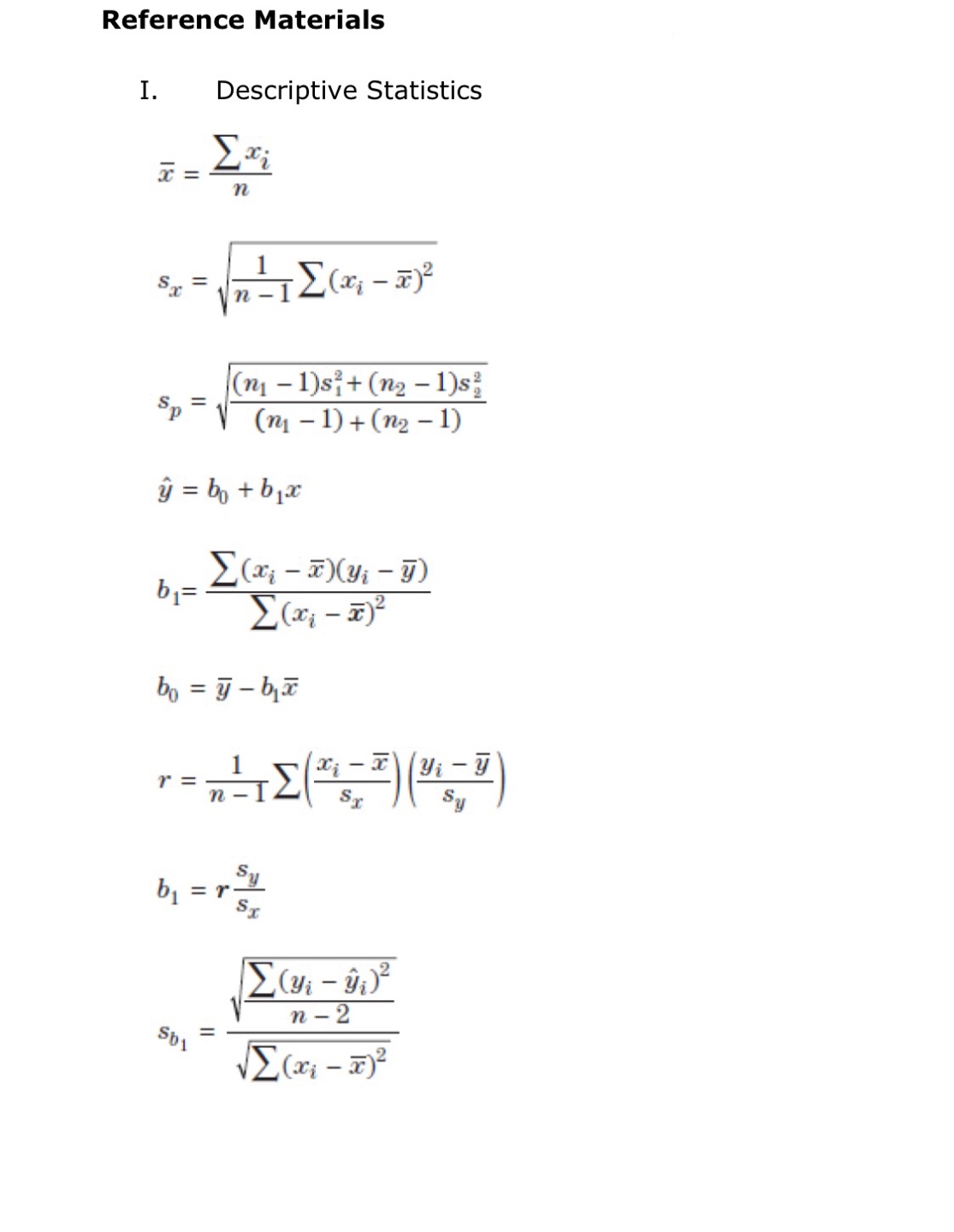
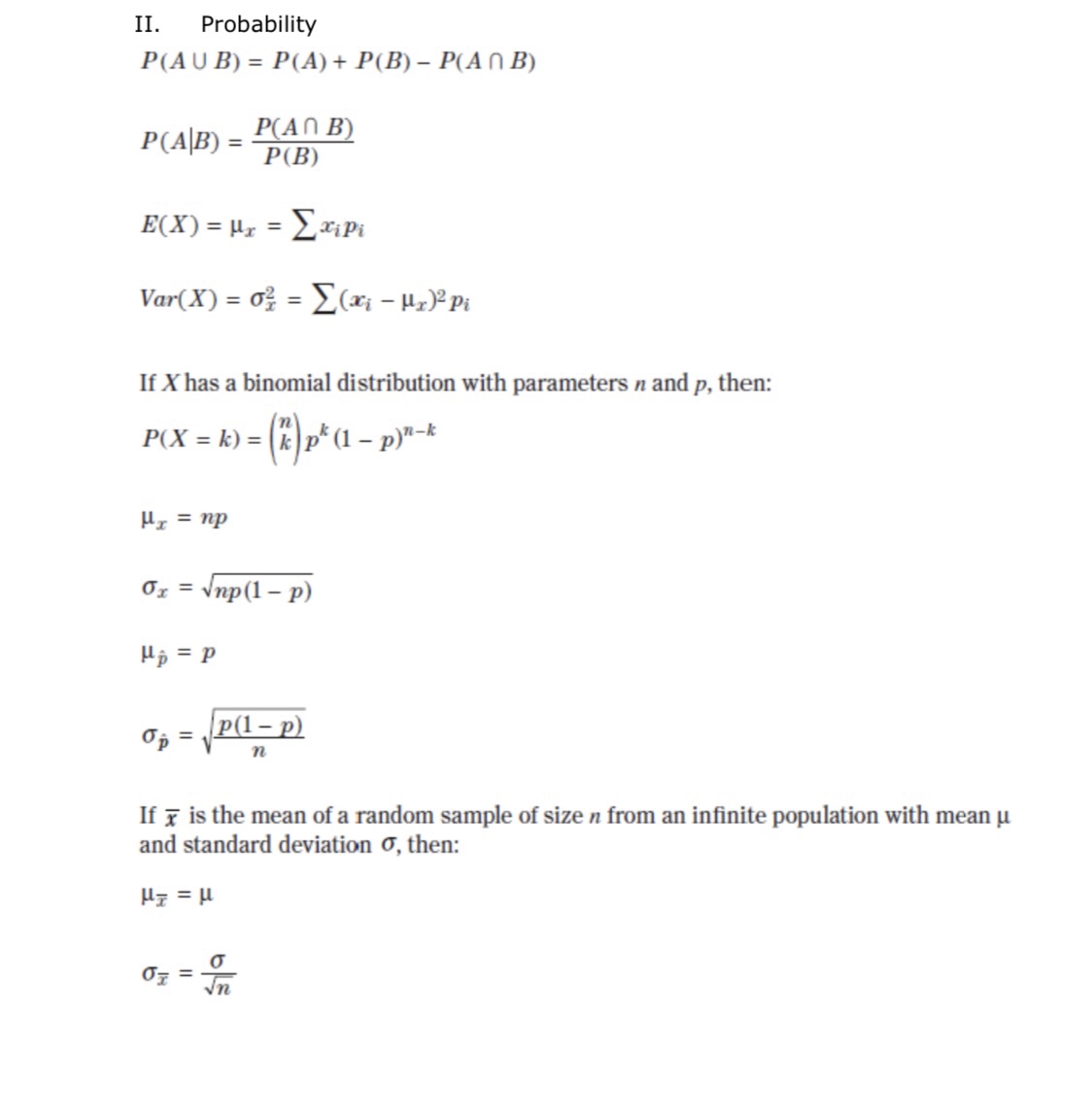
II. Probability P(AUB) = P(A) + P(B) - P(An B) P(AB) = P(An B) P(B) E(X) = Ux = Expi Var(X) = 0; = _(x - ux)2pi If X has a binomial distribution with parameters n and p, then: P(X = k) = k) p* (1 - p)" -* HI = np Or = Vnp(1 - p) Ho = P Op = P(1- p n If x is the mean of a random sample of size n from an infinite population with mean u and standard deviation O, then: MY = HIII. Inferential Statistics Standardized test statistic: statistic - parameter standard deviation of statistic Confidence interval: statistic + (critical value) . (standard deviation of statistic) Single-Sample Statistic Standard Deviation of Statistic Sample Mean Sample Proportion p(1 - p) n Two-Sample Statistic Standard Deviation of Statistic Difference of sample means 722 Special case when 61 =02 ol+1 n2 Difference of PI (1 - PI) + P2 (1 - P2) sample proportions n1 n2 Special case when P1 = P2 Jp(1 - P) 1 + 1 Vn, n2 Chi-square test statistic = \\ (observed - expected) expected\fTable entry for p and C is the point t* with probability p lying above it Probability p and probability C lying between -t* and t*. Table B t distribution critical values Tail probability p df .25 .20 .15 .10 05 .025 .02 .01 .005 0025 .001 .0005 1.000 1.376 1.963 3.078 6.314 12.71 15.89 31.82 63.66 127.3 318.3 636.6 .816 1.061 1.386 1.886 2.920 4.303 4.849 6.965 9.925 14.09 22.33 31.60 .765 978 1.250 1.638 2.353 3.182 3.482 4.541 5.841 7.453 10.21 12.92 .741 .941 1.190 1.533 2.132 2.776 2.999 3.747 4.604 5.598 7.173 8.610 .727 920 1.156 1.476 2.015 2.571 2.757 3.365 4.032 4.773 5.893 6.869 .718 906 1.134 1.440 1.943 2.447 2.612 3.143 3.707 4.317 5.208 5.959 .711 .896 1.119 1.415 1.895 2.365 2.517 2.998 3.499 4.029 4.785 5.408 .706 889 1.108 1.397 1.860 2.306 2.449 2.896 3.355 3.833 4.501 5.041 1703 883 1.100 1.383 1.833 2.262 2.398 2.821 3.250 3.690 4.297 4.781 10 700 879 1.093 1.372 1.812 2.228 2.359 2.764 3.169 3.581 4.144 4.587 .697 .876 1.088 1.363 1.796 2.201 2.328 2.718 3.106 3.497 4.025 4.437 12 695 873 1.083 1.356 1.782 2.179 2.303 2.681 3.055 3.428 3.930 4.318 13 694 870 1.079 1.350 1.771 2.160 2.282 2.650 3.012 3.372 3.852 4.221 14 .692 868 1.076 1.345 1.761 2.145 2.264 2.624 2.977 3.326 3.787 4.140 15 691 866 1.074 1.341 1.753 2.131 2.249 2.602 2.947 3.286 3.733 4.073 16 .690 865 1.071 1.337 1.746 2.120 2.235 2.583 2.921 3.252 3.686 4.015 689 863 1.069 1.333 1.740 2.110 2.224 2.567 2.898 3.222 3.646 3.965 18 688 862 1.067 1.330 1.734 2.101 2.214 2.552 2.878 3.197 3.611 3.922 19 .688 .861 1.066 1.328 1.729 2.093 2.205 2.539 2.861 3.174 3.579 3.883 20 687 860 1.064 1.325 1.725 2.086 2.197 2.528 2.845 3.153 3.552 3.850 21 686 859 1.063 1.323 1.721 2.080 2.189 2.518 2.831 3.135 3.527 3.819 686 .858 1.061 1.321 1.717 2.074 2.183 2.508 2.819 3.119 3.505 3.792 23 685 858 1.060 1.319 1.714 2.069 2.177 2.500 2.807 3.104 3.485 3.768 24 685 857 1.059 1.318 1.711 2.064 2.172 2.492 2.797 3.091 3.467 3.745 25 .684 856 1.058 1.316 1.708 2.060 2.167 2.485 2.787 3.078 3.450 3.725 26 .684 856 1058 1.315 1.706 2.056 2.162 2.479 2.779 3.067 3.435 3.707 27 684 855 1.057 1.314 1.703 2.052 2.158 2.473 2.771 3.057 3.421 3.690 28 683 855 1.056 1.313 1.701 2.048 2.154 2.467 2.763 3.047 3.408 3.674 29 683 .854 1.055 1.311 1.699 2.045 2.150 2.462 2.756 3.038 3.396 3.659 30 .683 .854 1.055 1.310 1.697 2.042 2.147 2.457 2.750 3.030 3.385 3.646 40 .681 .851 1.050 1.303 1.684 2.021 2.123 2.423 2.704 2.971 3.307 3.551 50 .679 .849 1.047 1.299 1.676 2.009 2.109 2.403 2.678 2.937 3.261 3.496 60 .679 .848 1.045 1.296 1.671 2.000 2.099 2.390 2.660 2.915 3.232 3.460 80 .678 .846 1.043 1.292 1.664 1.990 2.088 2.374 2.639 2.887 3.195 3.416 100 .677 .845 1.042 1.290 1.660 1.984 2.081 2.364 2.626 2.871 3.174 3.390 1000 .675 .842 1.037 1.282 1.646 1.962 2.056 2.330 2.581 2.813 3.098 3.300 .674 841 1.036 1.282 1.645 1.960 2.054 2.326 2.576 2.807 3.091 3.291 50% 60% 70% 80% 90% 95% 96% 98% 99% 99.5% 99.8% 99.9% Confidence level CTable entry Probability p for p is the point (x ) with probability p lying above it. (x2) Table C * critical values Tail probability p df .25 .20 .15 .10 05 025 .02 .01 .005 .0025 001 1 1.32 1.64 2.07 2.71 3.84 5.02 5.41 6.63 7.88 9.14 10.83 2.77 3.22 3.79 4.61 5.99 7.38 7.82 9.21 10.60 11.98 13.82 4.11 4.64 5.32 6.25 7.81 9.35 9.84 11.34 12.84 14.32 16.27 5.39 5.99 6.74 7.78 9.49 11.14 11.67 13.28 14.86 16.42 18.47 6.63 7.29 8.12 9.24 11.07 12.83 13.39 15.09 16.75 18.39 20.51 7.84 8.56 9.45 10.64 12.59 14.45 15.03 16.81 18.55 20.25 22.46 9.04 9.80 10.75 12.02 14.07 16.01 16.62 18.48 20.28 22.04 24.32 10.22 11.03 12.03 13.36 15.51 17.53 18.17 20.09 21.95 23.77 26.12 11.39 12.24 13.29 14.68 16.92 19.02 19.68 21.67 23.59 25.46 27.88 12.55 13.44 14.53 15.99 18.31 20.48 21.16 23.21 25.19 27.11 29.59 11 13.70 14.63 15.77 17.28 19.68 21.92 22.62 24.72 26.76 28.73 31.26 12 14.85 15.81 16.99 18.55 21.03 23.34 24.05 26.22 28.30 30.32 32.91 13 15.98 16.98 18.20 19.81 22.36 24.74 25.47 27.69 29.82 31.88 34.53 14 17.12 18.15 19.41 21.06 23.68 26.12 26.87 29.14 31.32 33.43 36.12 15 18.25 19.31 20.60 22.31 25.00 27.49 28.26 30.58 32.80 34.95 37.70 16 19.37 20.47 21.79 23.54 26.30 28.85 29.63 32.00 34.27 36.46 39.25 17 20.49 21.61 22.98 24.77 27.59 30.19 31.00 33.41 35.72 37.95 40.79 18 21.60 22.76 24.16 25.99 28.87 31.53 32.35 34.8 37.16 39.42 42.31 19 22.72 23.90 25.33 27.20 30.14 32.85 33.69 36.19 38.58 40.88 43.82 20 23.83 25.04 26.50 28.41 31.41 34.17 35.02 37.57 40.00 42.34 45.31 21 24.93 26.17 27.66 29.62 32.67 35.48 36.34 38.93 41.40 43.78 46.80 22 26.04 27.30 28.82 30.81 33.92 36.78 37.66 40.29 42.80 45.20 48.27 23 27.14 28.43 29.98 32.01 35.17 38.08 38.97 1.64 44.18 46.62 49.73 24 28.24 29.55 31.13 33.20 36.42 39.36 40.27 42.98 45.56 48.03 51.18 25 29.34 30.68 32.28 34.38 37.65 40.65 41.57 44.31 46.93 49.44 52.62 26 30.43 31.79 33.43 35.56 38.89 41.92 42.86 45.64 48.29 50.83 54.05 27 31.53 32.91 34.57 36.74 40.11 43.19 44.14 46.96 49.64 52.22 55.48 28 32.62 34.03 35.71 37.92 41.34 44.46 45.42 48.28 50.99 53.59 56.89 29 33.71 35.14 36.85 39.09 42.56 45.72 46.69 49.59 52.34 54.97 58.30 30 34.80 36.25 37.99 40.26 43.77 46.98 47.96 50.89 53.67 56.33 59.70 40 45.62 47.27 49.24 51.8 55.76 59.34 60.44 63.69 66.77 69.70 73.40 50 56.33 58.16 60.35 63.17 67.50 71.42 72.61 76.15 79.49 82.66 86.66 60 66.98 68.97 71.34 74.40 79.08 83.30 84.58 88.38 91.95 95.34 99.61 80 88.13 90.41 93.11 96.58 101.9 106.6 108.1 112.3 116.3 120.1 124.8 100 109.1 111.7 114.7 118.5 124.3 129.6 131.1 135.8 140.2 144.3 149.4D DIRECTIONS: Use this information for questions 21 and 22. Suppose it is known that in the United States 11% of men and 9% of women are left-handed. Imagine you are considering conducting your own random survey of 50 American men and 50 American women. D Question 21 1 pts What is the probability that your survey would find a higher proportion of left-handedness in women than in men? O 0.369 O 0.185 O 0.060 O 0.738 O 0.837D Question 22 1 pts You are considering doubling the number of participants in your survey to 100 men and 100 women. Which of these would be the most likely result of this decision? The probability of getting a difference in sample proportions is less likely to be closer to 0.02. The probability of getting a difference in sample proportions is more likely to be closer to 0.02. The probability of getting a difference in sample proportions is more likely to be closer to 11%. O The probability of getting a difference in sample proportions is more likely to be closer to 9% There is a reduced risk of error due to response bias.