This is the Table I need to complete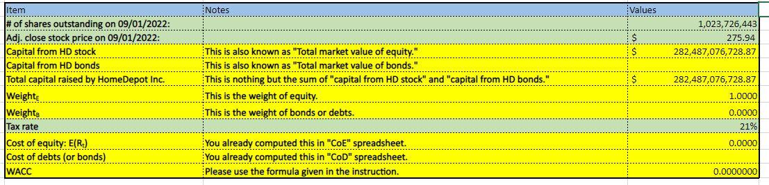

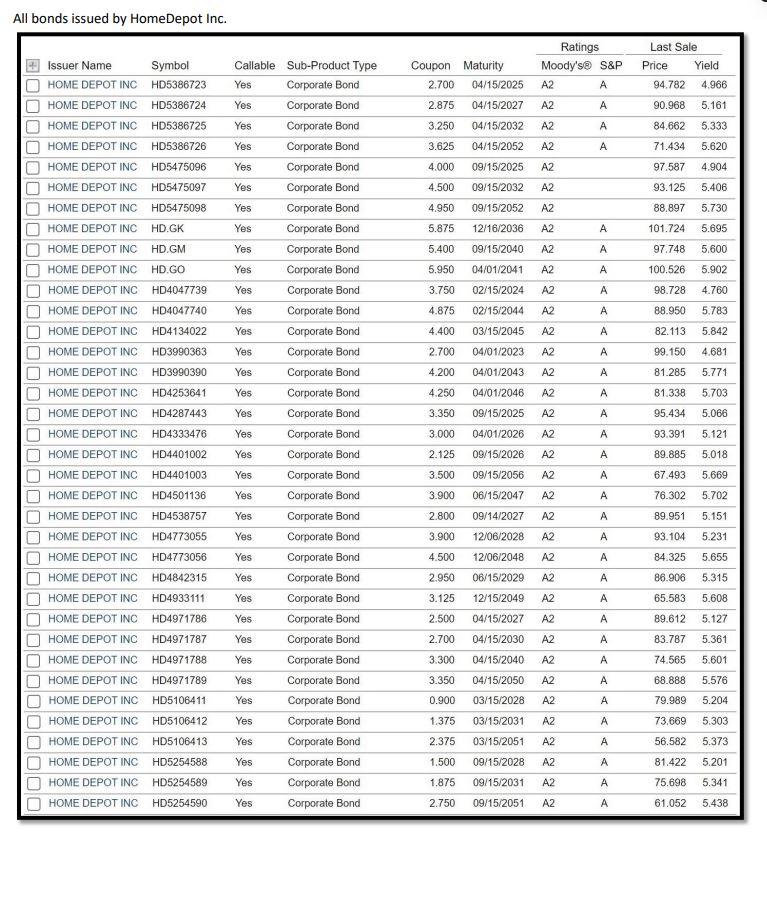
These are the files that were provided to solve the problem

This is an example of a completed Table

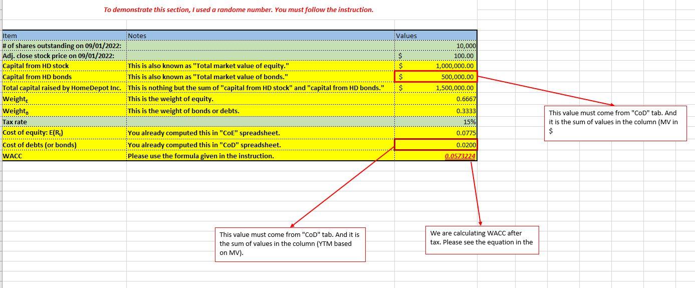
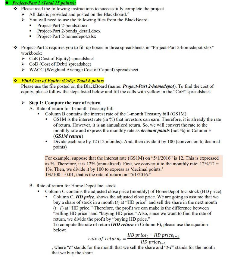
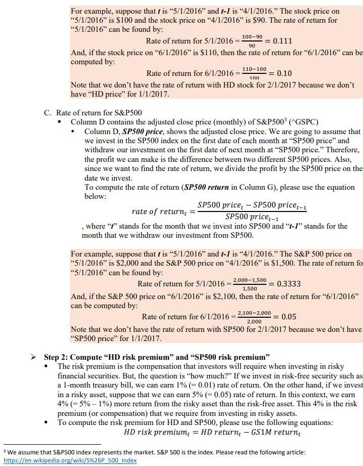
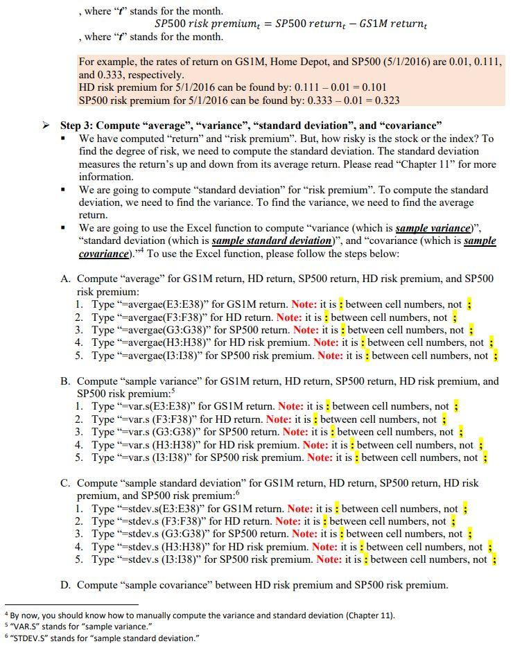
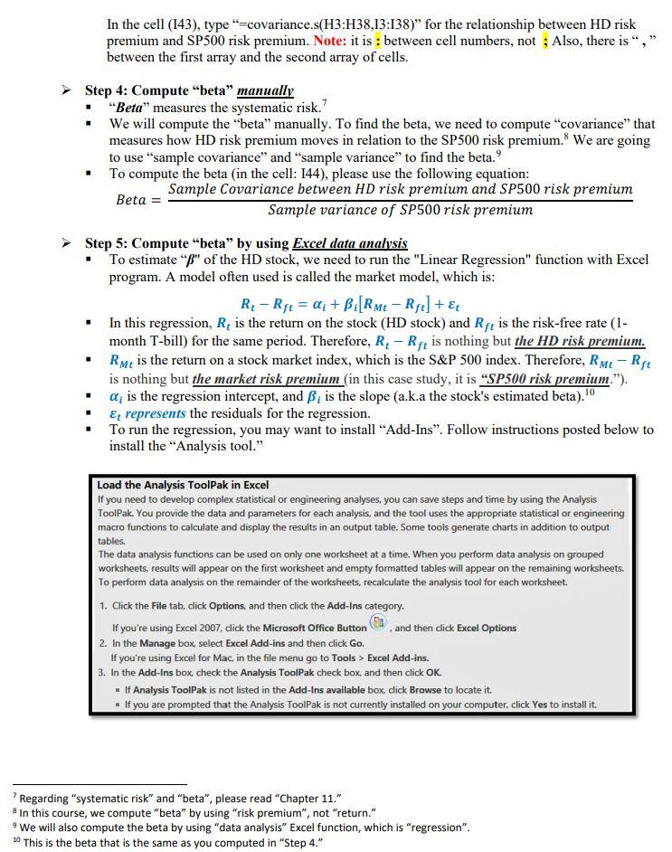
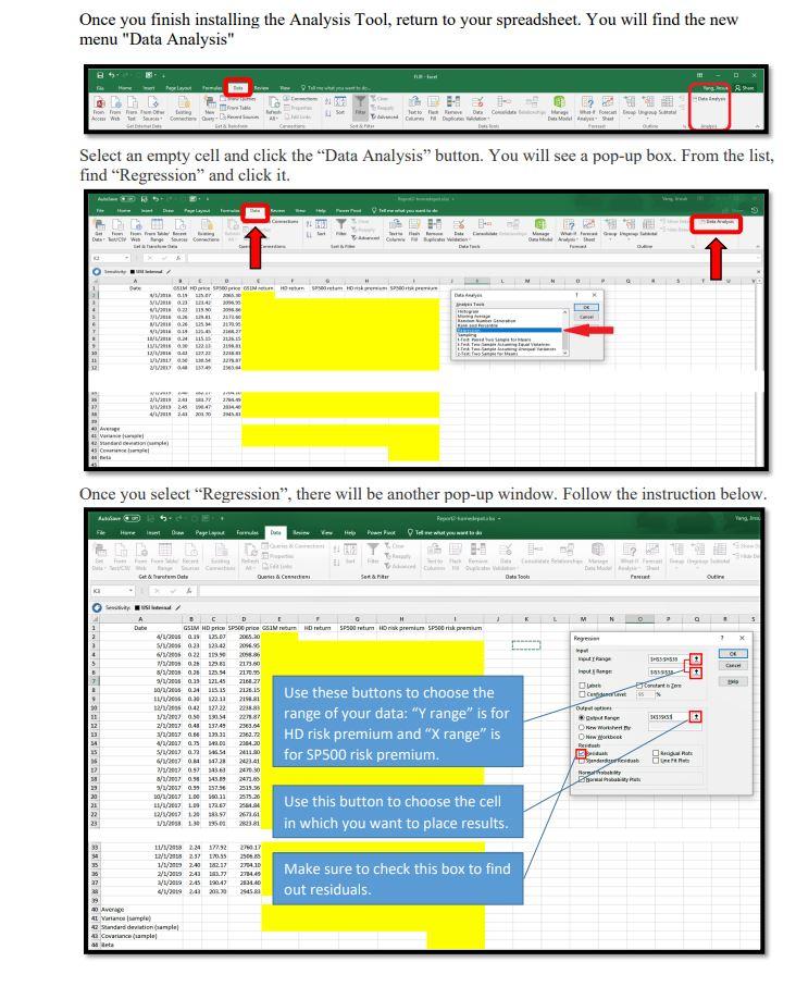
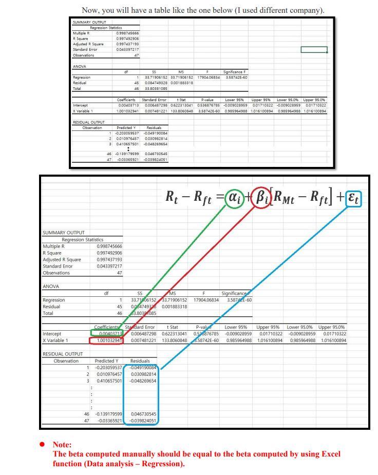
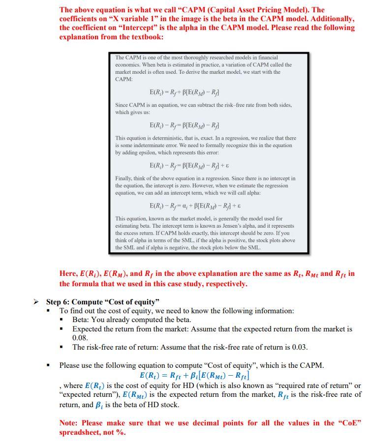
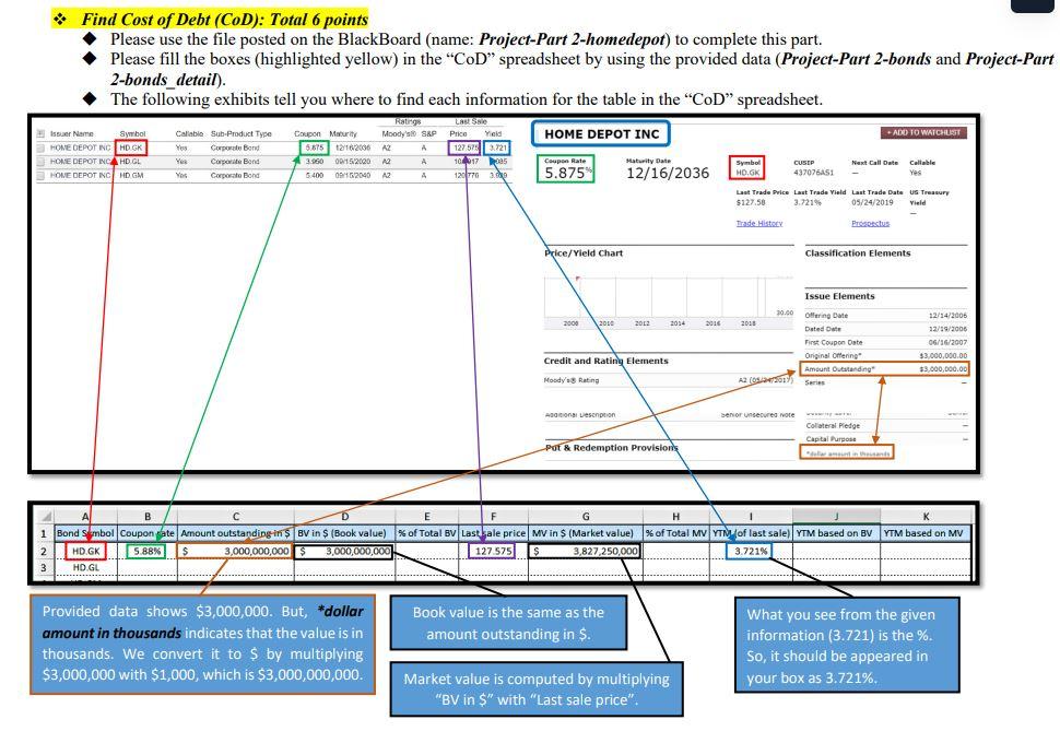
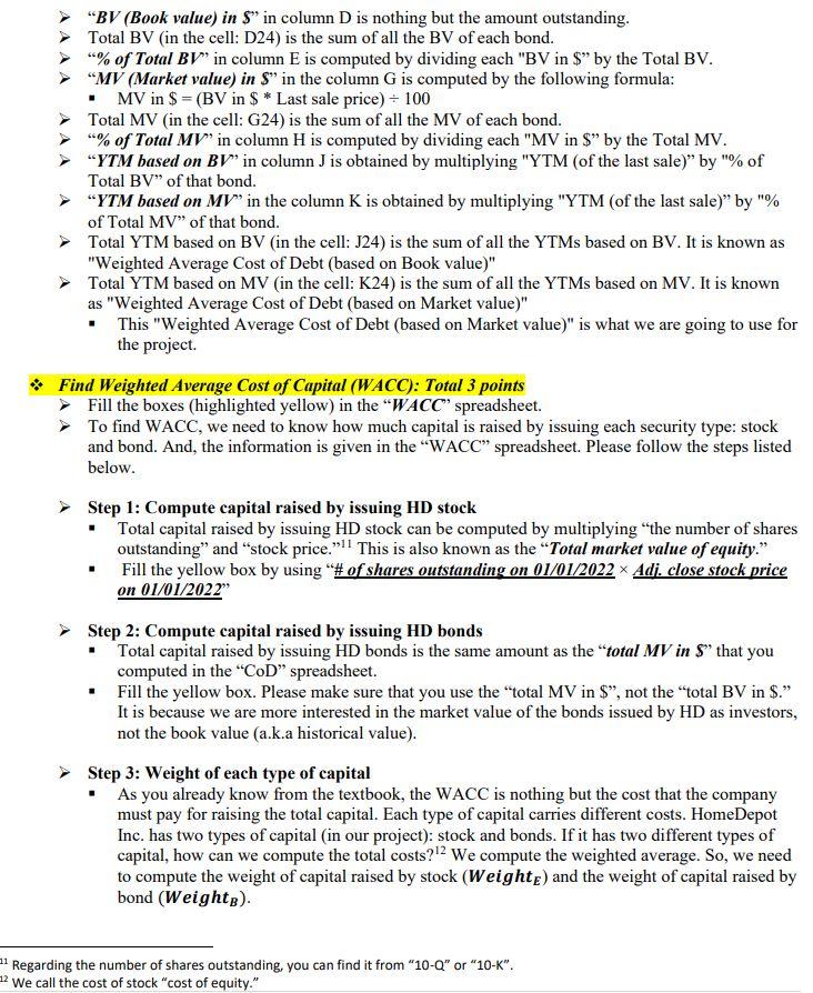
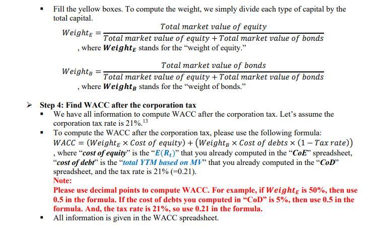
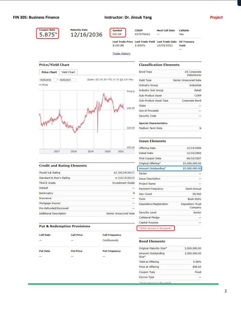
All bonds issued by HomeDepot Inc. Project-Part 2 (Total 15 points): * Please read the following instructions to successfully complete the project All data is provided and posted on the Blackboard. 2 You will need to use the following files from the BlackBoard. - Project-Part 2-bonds.docx - Project-Part 2-bonds detail.docx - Project-Part 2-homedepot.xlsx * Project-Part 2 requires you to fill up boxes in three spreadsheets in "Project-Part 2-homedepot.xlsx" workbook: CoE (Cost of Equity) spreadsheet CoD( Cost of Debt) spreadsheet WACC (Weighted Average Cost of Capital) spreadsheet * Find Cost of Equity (CoE): Total 6 points Please use the file posted on the BlackBoard (name: Project-Part 2-homedepot). To find the cost of equity, please follow the steps listed below and fill the cells with yellow in the "CoE" spreadsheet. Step 1: Compute the rate of return A. Rate of return for 1-month Treasury bill - Column B contains the interest rate of the 1-month Treasury bill (GS1M). - GS1M is the interest rate (in \%) that investors can earn. Therefore, it is already the rate of return. However, it is an annualized return. So, we will convert the rate to the monthly rate and express the monthly rate as decimal points (not \%) in Column E (GS1M return) - Divide each rate by 12 (12 months). And, then divide it by 100 (conversion to decimal points) For example, suppose that the interest rate (GS1M) on " 5/1/2016 " is 12 . This is expressed as %. Therefore, it is 12% (annualized). First, we convert it to the monthly rate: 12%/12= 1%. Then, we divide it by 100 to express as 'decimal points.' 1%/100=0.01, that is the rate of return on "5/1/2016." B. Rate of return for Home Depot Inc. stock - Column C contains the adjusted close price (monthly) of HomeDepot Inc. stock (HD price) - Column C, HD price, shows the adjusted close price. We are going to assume that we buy a share of stock in a month (t) at "HD price" and sell the share in the next month (t+l) at "HD price." Therefore, the profit we can make is the difference between "selling HD price" and "buying HD price." Also, since we want to find the rate of return, we divide the profit by "buying HD price." To compute the rate of return (HD return in Column F), please use the equation below: rateofreturnt=HDpricet1HDpricetHDpricet1 , where " t " stands for the month that we sell the share and " t1 " stands for the month that we buy the share. For example, suppose that t is " 5/1/2016 " and tI is " 4/1/2016." The stock price on " 5/1/2016 " is $100 and the stock price on " 4/1/2016 " is $90. The rate of return for " 5/1/2016 " can be found by: Rate of return for 5/1/2016=9010090=0.111 And, if the stock price on " 6/1/2016 " is $110, then the rate of return for " 6/1/2016 " can be computed by: Rate of return for 6/1/2016=10n110100=0.10 Note that we don't have the rate of return with HD stock for 2/1/2017 because we don't have "HD price" for 1/1/2017 C. Rate of return for S\&P500 - Column D contains the adjusted close price (monthly) of S\&P500 3 (^GSPC) - Column D, SP500 price, shows the adjusted close price. We are going to assume that we invest in the SP500 index on the first date of each month at "SP500 price" and withdraw our investment on the first date of next month at "SP500 price." Therefore, the profit we can make is the difference between two different SP500 prices. Also, since we want to find the rate of return, we divide the profit by the SP500 price on the date we invest. To compute the rate of return (SP500 return in Column G), please use the equation below: rateofreturnt=SP500pricet1SP500pricetSP500pricet1 , where " t " stands for the month that we invest into SP500 and " t1 " stands for the month that we withdraw our investment from SP500. For example, suppose that t is "5/1/2016" and t1 is "4/1/2016." The S\&P 500 price on "5/1/2016" is $2,000 and the S\&P 500 price on "4/1/2016" is $1,500. The rate of return fo " 5/1/2016 " can be found by: Rate of return for 5/1/2016=1,5002,0001,500=0.3333 And, if the S\&P 500 price on " 6/1/2016 " is $2,100, then the rate of return for " 6/1/2016 " can be computed by: Rate of return for 6/1/2016=2,0002,1002,000=0.05 Note that we don't have the rate of return with SP500 for 2/1/2017 because we don't have "SP500 price" for 1/1/2017. Step 2: Compute "HD risk premium" and "SP500 risk premium" - The risk premium is the compensation that investors will require when investing in risky financial securities. But, the question is "how much?" If we invest in risk-free security such as a 1-month treasury bill, we can earn 1%(=0.01) rate of return. On the other hand, if we invest in a risky asset, suppose that we can earn 5%(=0.05) rate of return. In this context, we earn 4%(=5%1%) more return from the risky asset than the risk-free asset. This 4% is the risk premium (or compensation) that we require from investing in risky assets. - To compute the risk premium for HD and SP500, please use the following equations: HD risk premium p t=HD return tGS1M return t 3 We assume that S\&P500 index represents the market. S\&P 500 is the index. Please read the following article: https://en.wikipedia.org/wiki/S\%26P 500 Index , where " t ' stands for the month. SP500 risk premium pret t=SP500 return tGS1 return t , where " t ' stands for the month. For example, the rates of return on GS1M, Home Depot, and SP500 (5/1/2016) are 0.01,0.111, and 0.333 , respectively. HD risk premium for 5/1/2016 can be found by: 0.1110.01=0.101 SP500 risk premium for 5/1/2016 can be found by: 0.3330.01=0.323 Step 3: Compute "average", "variance", "standard deviation", and "covariance" - We have computed "return" and "risk premium". But, how risky is the stock or the index? To find the degree of risk, we need to compute the standard deviation. The standard deviation measures the return's up and down from its average return. Please read "Chapter 11 " for more information. - We are going to compute "standard deviation" for "risk premium". To compute the standard deviation, we need to find the variance. To find the variance, we need to find the average return. - We are going to use the Excel function to compute "variance (which is sample variance)", "standard deviation (which is sample standard deviation)", and "covariance (which is sample covariance)." ," , use the Excel function, please follow the steps below: A. Compute "average" for GS1M return, HD return, SP500 return, HD risk premium, and SP500 risk premium: 1. Type "=avergae(E3:E38)" for GS1M return. Note: it is : between cell numbers, not ; 2. Type "=avergae(F3:F38)" for HD return. Note: it is : between cell numbers, not ; 3. Type "=avergae(G3:G38)" for SP500 return. Note: it is : between cell numbers, not ; 4. Type "=avergae (H3:H38) " for HD risk premium. Note: it is : between cell numbers, not ; 5. Type "=avergae(I3:I38)" for SP500 risk premium. Note: it is : between cell numbers, not ; B. Compute "sample variance" for GS1M return, HD return, SP500 return, HD risk premium, and SP500 risk premium: 5 1. Type "=var.s(E3:E38)" for GS1M return. Note: it is : between cell numbers, not ; 2. Type "=var.s (F3:F38)" for HD return. Note: it is : between cell numbers, not ; 3. Type "=var.s (G3:G38)" for SP500 return. Note: it is : between cell numbers, not ; 4. Type "=var.s (H3:H38)" for HD risk premium. Note: it is : between cell numbers, not ; 5. Type "=var.s (I3:I38)" for SP500 risk premium. Note: it is : between cell numbers, not ; C. Compute "sample standard deviation" for GS1M return, HD return, SP500 return, HD risk premium, and SP500 risk premium: 6 1. Type "=stdev.s(E3:E38)" for GS1M return. Note: it is : between cell numbers, not ; 2. Type "=stdev.s (F3:F38)" for HD return. Note: it is : between cell numbers, not ; 3. Type "=stdev.s (G3:G38)" for SP500 return. Note: it is : between cell numbers, not ; 4. Type "=stdev.s (H3:H38)" for HD risk premium. Note: it is : between cell numbers, not ; 5. Type "=stdev.s (I3:I38)" for SP500 risk premium. Note: it is : between cell numbers, not ; D. Compute "sample covariance" between HD risk premium and SP500 risk premium. 4 By now, you should know how to manually compute the variance and standard deviation (Chapter 11). " "VAR.S" stands for "sample variance." 6 "STDEV.S" stands for "sample standard deviation." In the cell (I43), type "=covariance.s(H3:H38,I3:I38)" for the relationship between HD risk premium and SP500 risk premium. Note: it is : between cell numbers, not ; Also, there is "," between the first array and the second array of cells. Step 4: Compute "beta" manually - "Beta" measures the systematic risk." - We will compute the "beta" manually. To find the beta, we need to compute "covariance" that measures how HD risk premium moves in relation to the SP500 risk premium. 8 We are going to use "sample covariance" and "sample variance" to find the beta. 9 - To compute the beta (in the cell: I44), please use the following equation: Beta =SamplevarianceofSP500riskpremiumSampleCovariancebetweenHDriskpremiumandSP500riskpremium Step 5: Compute "beta" by using Excel data analysis - To estimate " " of the HD stock, we need to run the "Linear Regression" function with Excel program. A model often used is called the market model, which is: RtRft=i+i[RMtRft]+t - In this regression, Rt is the return on the stock (HD stock) and Rft is the risk-free rate (1month T-bill) for the same period. Therefore, RtRft is nothing but the HD risk premium. - RMt is the return on a stock market index, which is the S\&P 500 index. Therefore, RMtRft is nothing but the market risk premium (in this case study, it is "SP500 risk premium."). - i is the regression intercept, and i is the slope (a.k.a the stock's estimated beta). 10 - t represents the residuals for the regression. - To run the regression, you may want to install "Add-Ins". Follow instructions posted below to install the "Analysis tool." Load the Analysis ToolPak in Excel If you need to develop complex statistical or engineering analyses, you can save steps and time by using the Analysis ToolPak. You provide the data and parameters for each analysis, and the tool uses the appropriate statistical or engineering macro functions to calculate and display the results in an output table. Some tools generate charts in addition to output tables. The data analysis functions can be used on only one worksheet at a time. When you perform data analysis on grouped worksheets, results will appear on the first worksheet and empty formatted tables will appear on the remaining worksheets. To perform data analysis on the remainder of the worksheets, recalculate the analysis tool for each worksheet. 1. Click the File tab, click Options, and then click the Add-Ins category. If you're using Excel 2007, click the Microsoft Office Button () , and then click Excel Options 2. In the Manage box, select Excel Add-ins and then click Go. If you're using Excel for Mac, in the file menu go to Tools > Excel Add-ins. 3. In the Add-Ins box, check the Analysis ToolPak check box, and then click OK. - If Analysis ToolPak is not listed in the Add-Ins available box click Browse to locate it. - If you are prompted that the Analysis ToolPak is not currently installed on your computer, click Yes to install it. "Regarding "systematic risk" and "beta", please read "Chapter 11." 8 In this course, we compute "beta" by using "risk premium", not "return." " We will also compute the beta by using "data analysis" Excel function, which is "regression". 10 This is the beta that is the same as you computed in "Step 4." Once you finish installing the Analysis Tool, return to your spreadsheet. You will find the new menu "Data Analysis" Select an empty cell and click the "Data Analysis" button. You will see a pop-up box. From the list, find "Regression" and click it. Now, you will have a table like the one below (I used different company). The beta computed manually should be equal to the beta computed by using Excel function (Data analysis-Regression). The above equation is what we call "CAPM (Capital Asset Pricing Model). The coefficients on "X variable 1 " in the image is the beta in the CAPM model. Additionally, the coefficient on "Intercept" is the alpha in the CAPM model. Please read the following explanation from the textbook: The CAPM is one of the most thoroughly researched models in financial economics. When beta is estimated in practice, a variation of CAPM called the market model is often used. To derive the market model, we start with the CAPM: E(Ri)=Rf+[E(RM)Rf] Since CAPM is an equation, we can subtract the risk-free rate from both sides, which gives us: E(Rj)Rf=[E(RM)Rf] This equation is deterministic, that is, exact. In a regression, we realize that there is some indeterminate error. We need to formally recognize this in the equation by adding epsilon, which represents this error: E(Ri)Rf=[E(RM)Rf]+ Finally, think of the above equation in a regression. Since there is no intercept in the equation, the intercept is zero. However, when we estimate the regression equation, we can add an intercept term, which we will call alpha: E(Ri)Rf=i+[E(RM)Rf]+ This equation, known as the market model, is generally the model used for estimating beta. The intercept term is known as Jensen's alpha, and it represents the excess return. If CAPM holds exactly, this intercept should be zero. If you think of alpha in terms of the SML, if the alpha is positive, the stock plots above the SML and if alpha is negative, the stock plots below the SML. Here, E(Ri),E(RM), and Rf in the above explanation are the same as Rt,RMt and Rft in the formula that we used in this case study, respectively. Step 6: Compute "Cost of equity" - To find out the cost of equity, we need to know the following information: - Beta: You already computed the beta. - Expected the return from the market: Assume that the expected return from the market is 0.08 . - The risk-free rate of return: Assume that the risk-free rate of return is 0.03 . - Please use the following equation to compute "Cost of equity", which is the CAPM. E(Rt)=Rft+i[E(RMt)Rft] , where E(Rt) is the cost of equity for HD (which is also known as "required rate of return" or "expected return"), E(RMt) is the expected return from the market, Rft is the risk-free rate of return, and i is the beta of HD stock. Note: Please make sure that we use decimal points for all the values in the "CoE" spreadsheet, not \%. *. Find Cost of Debt (CoD): Total 6 points - Please use the file posted on the BlackBoard (name: Project-Part 2-homedepot) to complete this part. Please fill the boxes (highlighted yellow) in the "CoD" spreadsheet by using the provided data (Project-Part 2-bonds and Project-Part 2-bonds detail). "BV (Book value) in $ " in column D is nothing but the amount outstanding. Total BV (in the cell: D24) is the sum of all the BV of each bond. "\% of Total B " in column E is computed by dividing each "BV in $ " by the Total BV. "MV (Market value) in $ " in the column G is computed by the following formula: - MV in $=(BV in $ Last sale price )100 Total MV (in the cell: G24) is the sum of all the MV of each bond. "\% of Total MV " in column H is computed by dividing each "MV in \$" by the Total MV. "YTM based on BV" in column J is obtained by multiplying "YTM (of the last sale)" by "\% of Total BV" of that bond. " YTM based on MV " in the column K is obtained by multiplying "YTM (of the last sale)" by "\% of Total MV" of that bond. Total YTM based on BV (in the cell: J24) is the sum of all the YTMs based on BV. It is known as "Weighted Average Cost of Debt (based on Book value)" Total YTM based on MV (in the cell: K24) is the sum of all the YTMs based on MV. It is known as "Weighted Average Cost of Debt (based on Market value)" - This "Weighted Average Cost of Debt (based on Market value)" is what we are going to use for the project. * Find Weighted Average Cost of Capital (WACC): Total 3 points Fill the boxes (highlighted yellow) in the "WACC' spreadsheet. To find WACC, we need to know how much capital is raised by issuing each security type: stock and bond. And, the information is given in the "WACC" spreadsheet. Please follow the steps listed below. Step 1: Compute capital raised by issuing HD stock - Total capital raised by issuing HD stock can be computed by multiplying "the number of shares outstanding" and "stock price."11 This is also known as the "Total market value of equity." - Fill the yellow box by using "\# of shares outstanding on 01/01/2022 Adi. close stock price on 01/01/2022 Step 2: Compute capital raised by issuing HD bonds - Total capital raised by issuing HD bonds is the same amount as the "total MV in $ " that you computed in the "CoD" spreadsheet. - Fill the yellow box. Please make sure that you use the "total MV in \$", not the "total BV in \$." It is because we are more interested in the market value of the bonds issued by HD as investors, not the book value (a.k.a historical value). Step 3: Weight of each type of capital - As you already know from the textbook, the WACC is nothing but the cost that the company must pay for raising the total capital. Each type of capital carries different costs. HomeDepot Inc. has two types of capital (in our project): stock and bonds. If it has two different types of capital, how can we compute the total costs? 12 We compute the weighted average. So, we need to compute the weight of capital raised by stock (WeightE) and the weight of capital raised by bond ( Weight BB). 11 Regarding the number of shares outstanding, you can find it from " 10Q or " 10K". 12 We call the cost of stock "cost of equity." - Fill the yellow boxes. To compute the weight, we simply divide each type of capital by the total capital. Weight E=Totalmarketvalueofequity+TotalmarketvalueofbondsTotalmarketvalueofequity , where Weight W stands for the "weight of equity." Weight B=Totalmarketvalueofequity+TotalmarketvalueofbondsTotalmarketvalueofbonds Step 4: Find WACC after the corporation tax - We have all information to compute WACC after the corporation tax. Let's assume the corporation tax rate is 21%.13 - To compute the WACC after the corporation tax, please use the following formula: "cost of debt" is the "total YTM based on MV" that you already computed in the "CoD" spreadsheet, and the tax rate is 21%(=0.21). Note: Please use decimal points to compute WACC. For example, if Weight E is 50%, then use 0.5 in the formula. If the cost of debts you computed in "CoD" is 5%, then use 0.5 in the formula. And, the tax rate is 21%, so use 0.21 in the formula. - All information is given in the WACC spreadsheet. Instructor: Dr. Jinsuk Yang LastTradePriceLi$140.882 To demonstrate this section, I used a randome number. You must follow the instruction. All bonds issued by HomeDepot Inc. Project-Part 2 (Total 15 points): * Please read the following instructions to successfully complete the project All data is provided and posted on the Blackboard. 2 You will need to use the following files from the BlackBoard. - Project-Part 2-bonds.docx - Project-Part 2-bonds detail.docx - Project-Part 2-homedepot.xlsx * Project-Part 2 requires you to fill up boxes in three spreadsheets in "Project-Part 2-homedepot.xlsx" workbook: CoE (Cost of Equity) spreadsheet CoD( Cost of Debt) spreadsheet WACC (Weighted Average Cost of Capital) spreadsheet * Find Cost of Equity (CoE): Total 6 points Please use the file posted on the BlackBoard (name: Project-Part 2-homedepot). To find the cost of equity, please follow the steps listed below and fill the cells with yellow in the "CoE" spreadsheet. Step 1: Compute the rate of return A. Rate of return for 1-month Treasury bill - Column B contains the interest rate of the 1-month Treasury bill (GS1M). - GS1M is the interest rate (in \%) that investors can earn. Therefore, it is already the rate of return. However, it is an annualized return. So, we will convert the rate to the monthly rate and express the monthly rate as decimal points (not \%) in Column E (GS1M return) - Divide each rate by 12 (12 months). And, then divide it by 100 (conversion to decimal points) For example, suppose that the interest rate (GS1M) on " 5/1/2016 " is 12 . This is expressed as %. Therefore, it is 12% (annualized). First, we convert it to the monthly rate: 12%/12= 1%. Then, we divide it by 100 to express as 'decimal points.' 1%/100=0.01, that is the rate of return on "5/1/2016." B. Rate of return for Home Depot Inc. stock - Column C contains the adjusted close price (monthly) of HomeDepot Inc. stock (HD price) - Column C, HD price, shows the adjusted close price. We are going to assume that we buy a share of stock in a month (t) at "HD price" and sell the share in the next month (t+l) at "HD price." Therefore, the profit we can make is the difference between "selling HD price" and "buying HD price." Also, since we want to find the rate of return, we divide the profit by "buying HD price." To compute the rate of return (HD return in Column F), please use the equation below: rateofreturnt=HDpricet1HDpricetHDpricet1 , where " t " stands for the month that we sell the share and " t1 " stands for the month that we buy the share. For example, suppose that t is " 5/1/2016 " and tI is " 4/1/2016." The stock price on " 5/1/2016 " is $100 and the stock price on " 4/1/2016 " is $90. The rate of return for " 5/1/2016 " can be found by: Rate of return for 5/1/2016=9010090=0.111 And, if the stock price on " 6/1/2016 " is $110, then the rate of return for " 6/1/2016 " can be computed by: Rate of return for 6/1/2016=10n110100=0.10 Note that we don't have the rate of return with HD stock for 2/1/2017 because we don't have "HD price" for 1/1/2017 C. Rate of return for S\&P500 - Column D contains the adjusted close price (monthly) of S\&P500 3 (^GSPC) - Column D, SP500 price, shows the adjusted close price. We are going to assume that we invest in the SP500 index on the first date of each month at "SP500 price" and withdraw our investment on the first date of next month at "SP500 price." Therefore, the profit we can make is the difference between two different SP500 prices. Also, since we want to find the rate of return, we divide the profit by the SP500 price on the date we invest. To compute the rate of return (SP500 return in Column G), please use the equation below: rateofreturnt=SP500pricet1SP500pricetSP500pricet1 , where " t " stands for the month that we invest into SP500 and " t1 " stands for the month that we withdraw our investment from SP500. For example, suppose that t is "5/1/2016" and t1 is "4/1/2016." The S\&P 500 price on "5/1/2016" is $2,000 and the S\&P 500 price on "4/1/2016" is $1,500. The rate of return fo " 5/1/2016 " can be found by: Rate of return for 5/1/2016=1,5002,0001,500=0.3333 And, if the S\&P 500 price on " 6/1/2016 " is $2,100, then the rate of return for " 6/1/2016 " can be computed by: Rate of return for 6/1/2016=2,0002,1002,000=0.05 Note that we don't have the rate of return with SP500 for 2/1/2017 because we don't have "SP500 price" for 1/1/2017. Step 2: Compute "HD risk premium" and "SP500 risk premium" - The risk premium is the compensation that investors will require when investing in risky financial securities. But, the question is "how much?" If we invest in risk-free security such as a 1-month treasury bill, we can earn 1%(=0.01) rate of return. On the other hand, if we invest in a risky asset, suppose that we can earn 5%(=0.05) rate of return. In this context, we earn 4%(=5%1%) more return from the risky asset than the risk-free asset. This 4% is the risk premium (or compensation) that we require from investing in risky assets. - To compute the risk premium for HD and SP500, please use the following equations: HD risk premium p t=HD return tGS1M return t 3 We assume that S\&P500 index represents the market. S\&P 500 is the index. Please read the following article: https://en.wikipedia.org/wiki/S\%26P 500 Index , where " t ' stands for the month. SP500 risk premium pret t=SP500 return tGS1 return t , where " t ' stands for the month. For example, the rates of return on GS1M, Home Depot, and SP500 (5/1/2016) are 0.01,0.111, and 0.333 , respectively. HD risk premium for 5/1/2016 can be found by: 0.1110.01=0.101 SP500 risk premium for 5/1/2016 can be found by: 0.3330.01=0.323 Step 3: Compute "average", "variance", "standard deviation", and "covariance" - We have computed "return" and "risk premium". But, how risky is the stock or the index? To find the degree of risk, we need to compute the standard deviation. The standard deviation measures the return's up and down from its average return. Please read "Chapter 11 " for more information. - We are going to compute "standard deviation" for "risk premium". To compute the standard deviation, we need to find the variance. To find the variance, we need to find the average return. - We are going to use the Excel function to compute "variance (which is sample variance)", "standard deviation (which is sample standard deviation)", and "covariance (which is sample covariance)." ," , use the Excel function, please follow the steps below: A. Compute "average" for GS1M return, HD return, SP500 return, HD risk premium, and SP500 risk premium: 1. Type "=avergae(E3:E38)" for GS1M return. Note: it is : between cell numbers, not ; 2. Type "=avergae(F3:F38)" for HD return. Note: it is : between cell numbers, not ; 3. Type "=avergae(G3:G38)" for SP500 return. Note: it is : between cell numbers, not ; 4. Type "=avergae (H3:H38) " for HD risk premium. Note: it is : between cell numbers, not ; 5. Type "=avergae(I3:I38)" for SP500 risk premium. Note: it is : between cell numbers, not ; B. Compute "sample variance" for GS1M return, HD return, SP500 return, HD risk premium, and SP500 risk premium: 5 1. Type "=var.s(E3:E38)" for GS1M return. Note: it is : between cell numbers, not ; 2. Type "=var.s (F3:F38)" for HD return. Note: it is : between cell numbers, not ; 3. Type "=var.s (G3:G38)" for SP500 return. Note: it is : between cell numbers, not ; 4. Type "=var.s (H3:H38)" for HD risk premium. Note: it is : between cell numbers, not ; 5. Type "=var.s (I3:I38)" for SP500 risk premium. Note: it is : between cell numbers, not ; C. Compute "sample standard deviation" for GS1M return, HD return, SP500 return, HD risk premium, and SP500 risk premium: 6 1. Type "=stdev.s(E3:E38)" for GS1M return. Note: it is : between cell numbers, not ; 2. Type "=stdev.s (F3:F38)" for HD return. Note: it is : between cell numbers, not ; 3. Type "=stdev.s (G3:G38)" for SP500 return. Note: it is : between cell numbers, not ; 4. Type "=stdev.s (H3:H38)" for HD risk premium. Note: it is : between cell numbers, not ; 5. Type "=stdev.s (I3:I38)" for SP500 risk premium. Note: it is : between cell numbers, not ; D. Compute "sample covariance" between HD risk premium and SP500 risk premium. 4 By now, you should know how to manually compute the variance and standard deviation (Chapter 11). " "VAR.S" stands for "sample variance." 6 "STDEV.S" stands for "sample standard deviation." In the cell (I43), type "=covariance.s(H3:H38,I3:I38)" for the relationship between HD risk premium and SP500 risk premium. Note: it is : between cell numbers, not ; Also, there is "," between the first array and the second array of cells. Step 4: Compute "beta" manually - "Beta" measures the systematic risk." - We will compute the "beta" manually. To find the beta, we need to compute "covariance" that measures how HD risk premium moves in relation to the SP500 risk premium. 8 We are going to use "sample covariance" and "sample variance" to find the beta. 9 - To compute the beta (in the cell: I44), please use the following equation: Beta =SamplevarianceofSP500riskpremiumSampleCovariancebetweenHDriskpremiumandSP500riskpremium Step 5: Compute "beta" by using Excel data analysis - To estimate " " of the HD stock, we need to run the "Linear Regression" function with Excel program. A model often used is called the market model, which is: RtRft=i+i[RMtRft]+t - In this regression, Rt is the return on the stock (HD stock) and Rft is the risk-free rate (1month T-bill) for the same period. Therefore, RtRft is nothing but the HD risk premium. - RMt is the return on a stock market index, which is the S\&P 500 index. Therefore, RMtRft is nothing but the market risk premium (in this case study, it is "SP500 risk premium."). - i is the regression intercept, and i is the slope (a.k.a the stock's estimated beta). 10 - t represents the residuals for the regression. - To run the regression, you may want to install "Add-Ins". Follow instructions posted below to install the "Analysis tool." Load the Analysis ToolPak in Excel If you need to develop complex statistical or engineering analyses, you can save steps and time by using the Analysis ToolPak. You provide the data and parameters for each analysis, and the tool uses the appropriate statistical or engineering macro functions to calculate and display the results in an output table. Some tools generate charts in addition to output tables. The data analysis functions can be used on only one worksheet at a time. When you perform data analysis on grouped worksheets, results will appear on the first worksheet and empty formatted tables will appear on the remaining worksheets. To perform data analysis on the remainder of the worksheets, recalculate the analysis tool for each worksheet. 1. Click the File tab, click Options, and then click the Add-Ins category. If you're using Excel 2007, click the Microsoft Office Button () , and then click Excel Options 2. In the Manage box, select Excel Add-ins and then click Go. If you're using Excel for Mac, in the file menu go to Tools > Excel Add-ins. 3. In the Add-Ins box, check the Analysis ToolPak check box, and then click OK. - If Analysis ToolPak is not listed in the Add-Ins available box click Browse to locate it. - If you are prompted that the Analysis ToolPak is not currently installed on your computer, click Yes to install it. "Regarding "systematic risk" and "beta", please read "Chapter 11." 8 In this course, we compute "beta" by using "risk premium", not "return." " We will also compute the beta by using "data analysis" Excel function, which is "regression". 10 This is the beta that is the same as you computed in "Step 4." Once you finish installing the Analysis Tool, return to your spreadsheet. You will find the new menu "Data Analysis" Select an empty cell and click the "Data Analysis" button. You will see a pop-up box. From the list, find "Regression" and click it. Now, you will have a table like the one below (I used different company). The beta computed manually should be equal to the beta computed by using Excel function (Data analysis-Regression). The above equation is what we call "CAPM (Capital Asset Pricing Model). The coefficients on "X variable 1 " in the image is the beta in the CAPM model. Additionally, the coefficient on "Intercept" is the alpha in the CAPM model. Please read the following explanation from the textbook: The CAPM is one of the most thoroughly researched models in financial economics. When beta is estimated in practice, a variation of CAPM called the market model is often used. To derive the market model, we start with the CAPM: E(Ri)=Rf+[E(RM)Rf] Since CAPM is an equation, we can subtract the risk-free rate from both sides, which gives us: E(Rj)Rf=[E(RM)Rf] This equation is deterministic, that is, exact. In a regression, we realize that there is some indeterminate error. We need to formally recognize this in the equation by adding epsilon, which represents this error: E(Ri)Rf=[E(RM)Rf]+ Finally, think of the above equation in a regression. Since there is no intercept in the equation, the intercept is zero. However, when we estimate the regression equation, we can add an intercept term, which we will call alpha: E(Ri)Rf=i+[E(RM)Rf]+ This equation, known as the market model, is generally the model used for estimating beta. The intercept term is known as Jensen's alpha, and it represents the excess return. If CAPM holds exactly, this intercept should be zero. If you think of alpha in terms of the SML, if the alpha is positive, the stock plots above the SML and if alpha is negative, the stock plots below the SML. Here, E(Ri),E(RM), and Rf in the above explanation are the same as Rt,RMt and Rft in the formula that we used in this case study, respectively. Step 6: Compute "Cost of equity" - To find out the cost of equity, we need to know the following information: - Beta: You already computed the beta. - Expected the return from the market: Assume that the expected return from the market is 0.08 . - The risk-free rate of return: Assume that the risk-free rate of return is 0.03 . - Please use the following equation to compute "Cost of equity", which is the CAPM. E(Rt)=Rft+i[E(RMt)Rft] , where E(Rt) is the cost of equity for HD (which is also known as "required rate of return" or "expected return"), E(RMt) is the expected return from the market, Rft is the risk-free rate of return, and i is the beta of HD stock. Note: Please make sure that we use decimal points for all the values in the "CoE" spreadsheet, not \%. *. Find Cost of Debt (CoD): Total 6 points - Please use the file posted on the BlackBoard (name: Project-Part 2-homedepot) to complete this part. Please fill the boxes (highlighted yellow) in the "CoD" spreadsheet by using the provided data (Project-Part 2-bonds and Project-Part 2-bonds detail). "BV (Book value) in $ " in column D is nothing but the amount outstanding. Total BV (in the cell: D24) is the sum of all the BV of each bond. "\% of Total B " in column E is computed by dividing each "BV in $ " by the Total BV. "MV (Market value) in $ " in the column G is computed by the following formula: - MV in $=(BV in $ Last sale price )100 Total MV (in the cell: G24) is the sum of all the MV of each bond. "\% of Total MV " in column H is computed by dividing each "MV in \$" by the Total MV. "YTM based on BV" in column J is obtained by multiplying "YTM (of the last sale)" by "\% of Total BV" of that bond. " YTM based on MV " in the column K is obtained by multiplying "YTM (of the last sale)" by "\% of Total MV" of that bond. Total YTM based on BV (in the cell: J24) is the sum of all the YTMs based on BV. It is known as "Weighted Average Cost of Debt (based on Book value)" Total YTM based on MV (in the cell: K24) is the sum of all the YTMs based on MV. It is known as "Weighted Average Cost of Debt (based on Market value)" - This "Weighted Average Cost of Debt (based on Market value)" is what we are going to use for the project. * Find Weighted Average Cost of Capital (WACC): Total 3 points Fill the boxes (highlighted yellow) in the "WACC' spreadsheet. To find WACC, we need to know how much capital is raised by issuing each security type: stock and bond. And, the information is given in the "WACC" spreadsheet. Please follow the steps listed below. Step 1: Compute capital raised by issuing HD stock - Total capital raised by issuing HD stock can be computed by multiplying "the number of shares outstanding" and "stock price."11 This is also known as the "Total market value of equity." - Fill the yellow box by using "\# of shares outstanding on 01/01/2022 Adi. close stock price on 01/01/2022 Step 2: Compute capital raised by issuing HD bonds - Total capital raised by issuing HD bonds is the same amount as the "total MV in $ " that you computed in the "CoD" spreadsheet. - Fill the yellow box. Please make sure that you use the "total MV in \$", not the "total BV in \$." It is because we are more interested in the market value of the bonds issued by HD as investors, not the book value (a.k.a historical value). Step 3: Weight of each type of capital - As you already know from the textbook, the WACC is nothing but the cost that the company must pay for raising the total capital. Each type of capital carries different costs. HomeDepot Inc. has two types of capital (in our project): stock and bonds. If it has two different types of capital, how can we compute the total costs? 12 We compute the weighted average. So, we need to compute the weight of capital raised by stock (WeightE) and the weight of capital raised by bond ( Weight BB). 11 Regarding the number of shares outstanding, you can find it from " 10Q or " 10K". 12 We call the cost of stock "cost of equity." - Fill the yellow boxes. To compute the weight, we simply divide each type of capital by the total capital. Weight E=Totalmarketvalueofequity+TotalmarketvalueofbondsTotalmarketvalueofequity , where Weight W stands for the "weight of equity." Weight B=Totalmarketvalueofequity+TotalmarketvalueofbondsTotalmarketvalueofbonds Step 4: Find WACC after the corporation tax - We have all information to compute WACC after the corporation tax. Let's assume the corporation tax rate is 21%.13 - To compute the WACC after the corporation tax, please use the following formula: "cost of debt" is the "total YTM based on MV" that you already computed in the "CoD" spreadsheet, and the tax rate is 21%(=0.21). Note: Please use decimal points to compute WACC. For example, if Weight E is 50%, then use 0.5 in the formula. If the cost of debts you computed in "CoD" is 5%, then use 0.5 in the formula. And, the tax rate is 21%, so use 0.21 in the formula. - All information is given in the WACC spreadsheet. Instructor: Dr. Jinsuk Yang LastTradePriceLi$140.882 To demonstrate this section, I used a randome number. You must follow the instruction