This model that the question references is this:

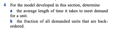
4 For the model developed in this section, determine a the average length of time it takes to meet demand for a unit b the fraction of all demanded units that are back- ordered. M FIGURE 12 Evolution of Inventory aver Time for E0Q Model with Back Orders Allowed D 0 C I 4-M We assume that the lead time for each order is zero. Since an order is placed each time the firm is q - Munits short (or when the firms inventory position is M - 9), the firm's maximum inventory level will be M - 4+4 = M. For example, if q = 500 and q - M= 100, we know that an order for 500 units will be used to satisfy the backlogged demand for 100 units and will result in an inventory level of 500 100 = 400 units. Assuming that an order is placed at time 0, the evolution of the inventory level over time is described by Figure 12. Since purchasing costs do not depend on q and M, we can minimize annual costs by determining the values of q and M that minimize Holding cost shortage cost order cost (9) year Notice that what happens between time and time B is identical to what happens be- tween time B and time D. For this reason, we call the time periods 0B and BD cycles. A cycle may also be thought of as the time interval between placement of orders. To deter- mine holding cost per year and shortage cost per year, we begin by finding holding cost per cycle and shortage cost per cycle. This requires that we find the length of line seg- ments 0A and AB in Figure 12. Since a zero inventory level occurs after Munits have been demanded, we conclude that 04 = Since a cycle ends when q units have been de- manded, we conclude that OB = . Then Length of AB = (length of 0B) - (length of 04) = D Also note that since q units are ordered during each cycle, cycles (and orders) must be placed during each year. We can now express the costs in (9). Recall that Holding cost holding cost cycles cycle year and Holding cost holding cost from time 0 to time A Cycle From Figure 12, the average inventory level between time and time A is simply. Since 04 is of length Holding cost M Mh Cycle D D 9 D q-M (*) (*) 2 2D ()- - 2D s) 4 {(1-1)(4M). - 19-20 D 2D Since there are cycles per year, Holding cost Mh 29 Similarly, Shortage cost shortage cost cycles cycle year Also observe that shortage cost per cycle = shortage cost incurred during time AB. Since demand occurs at a constant rate, the average shortage level during time AB is simply half of the maximum shortage. Thus, the average shortage level on the time interval AB is Since AB is a time interval of length, Shortage cost M Cycle 2 2D Since there are cycles per year, Shortage cost (q - M)'s D @ (q - Mos 24 As usual, ordering cost per year Let TCY, M) be the total annual cost (excluding purchasing cost) if our order policy uses parameters and M. From our discussion, we 4 must choose q and M to minimize Mh (9- Ms KD TC4, M) = 29 24 9 By using Theorem 3 of Chapter 11, we can show that TC(q, M) is a convex function of , and M. From Theorem l' and Theorem 7 of Chapter 11, the minimum value of TCC7, M) will occur at the point where aTC aTC Some tedious algebra shows that TC(q, M) is minimized for q* and M*: 2KD(+8) h + = hs 2KDs 11/2 M = = EOQ hh + 8)) h+ Maximum shortage = q* - M KD 9 + = 0 2 1/2 s +9]'* = EOQ ("#)" be (hts) 1/2