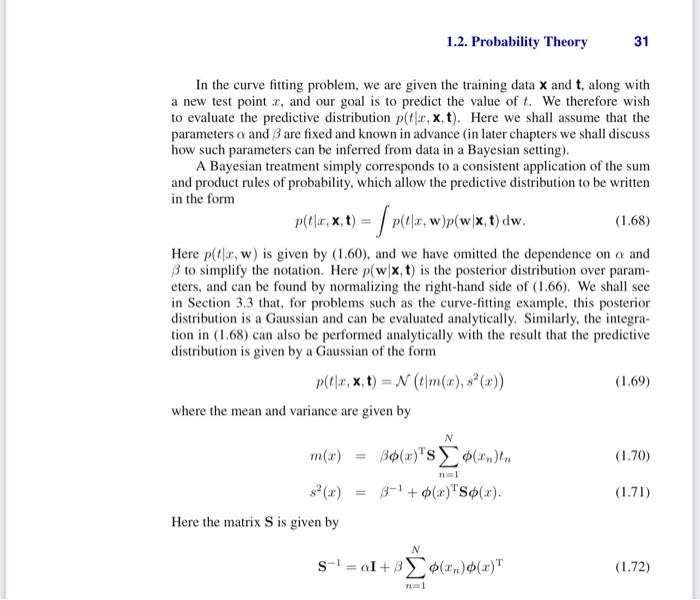
This page is taken from Bishop Springer, Pattern Recognition and Machine Learning. Please help me to derive and prove equation 1.70, 1.71 and 1.72 from 1.69.

In the curve fitting problem, we are given the training data X and t, along with a new test point x, and our goal is to predict the value of t. We therefore wish to evaluate the predictive distribution p(tx,x,t). Here we shall assume that the parameters and are fixed and known in advance (in later chapters we shall discuss how such parameters can be inferred from data in a Bayesian setting). A Bayesian treatment simply corresponds to a consistent application of the sum and product rules of probability, which allow the predictive distribution to be written in the form p(tx,x,t)=p(tx,w)p(wx,t)dw. Here p(tx,w) is given by (1.60), and we have omitted the dependence on and to simplify the notation. Here p(wx,t) is the posterior distribution over parameters, and can be found by normalizing the right-hand side of (1.66). We shall see in Section 3.3 that, for problems such as the curve-fitting example, this posterior distribution is a Gaussian and can be evaluated analytically. Similarly, the integration in ( 1.68) can also be performed analytically with the result that the predictive distribution is given by a Gaussian of the form p(tx,x,t)=N(tm(x),s2(x)) where the mean and variance are given by m(x)=(x)TSn=1N(xn)tns2(x)=1+(x)TS(x). Here the matrix S is given by S1=I+n=1N(xn)(x)T In the curve fitting problem, we are given the training data X and t, along with a new test point x, and our goal is to predict the value of t. We therefore wish to evaluate the predictive distribution p(tx,x,t). Here we shall assume that the parameters and are fixed and known in advance (in later chapters we shall discuss how such parameters can be inferred from data in a Bayesian setting). A Bayesian treatment simply corresponds to a consistent application of the sum and product rules of probability, which allow the predictive distribution to be written in the form p(tx,x,t)=p(tx,w)p(wx,t)dw. Here p(tx,w) is given by (1.60), and we have omitted the dependence on and to simplify the notation. Here p(wx,t) is the posterior distribution over parameters, and can be found by normalizing the right-hand side of (1.66). We shall see in Section 3.3 that, for problems such as the curve-fitting example, this posterior distribution is a Gaussian and can be evaluated analytically. Similarly, the integration in ( 1.68) can also be performed analytically with the result that the predictive distribution is given by a Gaussian of the form p(tx,x,t)=N(tm(x),s2(x)) where the mean and variance are given by m(x)=(x)TSn=1N(xn)tns2(x)=1+(x)TS(x). Here the matrix S is given by S1=I+n=1N(xn)(x)T