This question comes from a problem set in my class Monte Carlo Methods and it uses Matlab

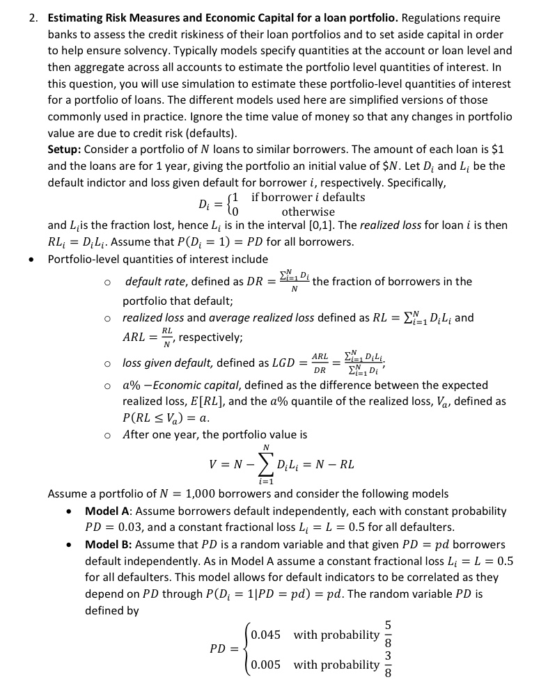
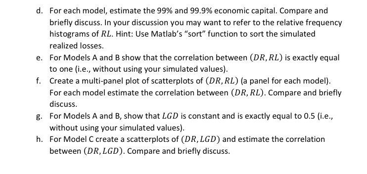
2. Estimating Risk Measures and Economic l[Zapital for a loan portfolio. Regulations require banks to assess the credit riskiness of their loan portfolios and to set aside capital in order to help ensure solvency. Typically models specify quantities at the account or loan level and then aggregate across all accounts to estimate the portfolio level quantities of interest. In this question, you will use simulation to estimate these portfoliolevel quantities ofinterest for a portfolio of loans. The different models used here are simplified versions of those commonly used in practice. Ignore the time value of money so that any changes in portfolio value are due to credit risk {defaults}. Setup: Consider a portfolio of N loans to similar borrowers. The amount of each loan is $1 and the loans are for 1 year, giving the portfolio an initial value of SN. Let DI and L1 be the default indictor and loss given default for borrower :3, respectively. Specifically, 1 if borroweri defaults Di = { 0 otherwise and Lyis the fraction lost, hence L! is in the interval [0,1]. The reoffzed foss for loan :2 is then RL, = 0112;. Assume that P-(Dy = 1} = PD for all borrowers. I Portfoliolevel quantities of interest include N o defouft rote, defined as DR = Elli- the fraction of borrowers in the portfolio that default; 0 reoffzedfoss and average reoffzedfoss defined as RL = 21 0,0! and RL . ARI. = F' respectively; Al 0 foss given defouft, defined as LSD = = Eli': DR 21-1-01 0 [1% Economic cop-ital, defined as the difference between the expected realized loss, E[RL], and the [1% quantile of the realized loss, if,\" defined as P(RL E 12;) = o. C:- After one year, the portfolio value is N V=NZD,L,=NRL [=1 Assume a portfolio ofN = 1,000 borrowers and consider the following models I Model A: Assume borrowers default independently, each with constant probability PD = 0.03, and a constant fractional loss L, = L = 0.5 for all defaulters. I Model B: Assume that PD is a random variable and that given PD = pd borrowers default independently. As in Model A assume a constant fractional loss L; = L = 0.5 for all defaulters. This model allows for default indicators to be correlated as they depend on PD through P'EDI = II?!) = pd) = pd. The random variable PD is defined by 5 0.045 with probability 5 3 0.005 with probability 5 PD: h. For each model, estimate the 99% and 99.9% economic capital. Compare and briefly discuss. In your discussion you may want to refer to the relative frequency histograms of RL. Hint: Use Matlab's "sort" function to sort the simulated realized losses. For Models A and B show that the correlation between (DR. RE.) is exactly equal to one {i.e., without using your simulated yalues}. Create a multipanel plot of scatterplots of (DE, EL) {a panel for each model}. For each model estimate the correlation between (DR, RL). Compare and briefly discuss. For Models A and B, show that LED is constant and is exactly equal to 0.5 {i.e., without using your simulated values]. For Model C create a scatterplots of (DELHI?!) and estimate the correlation between (DELHI?) Compare and briefly discuss