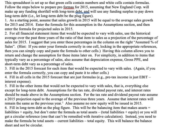
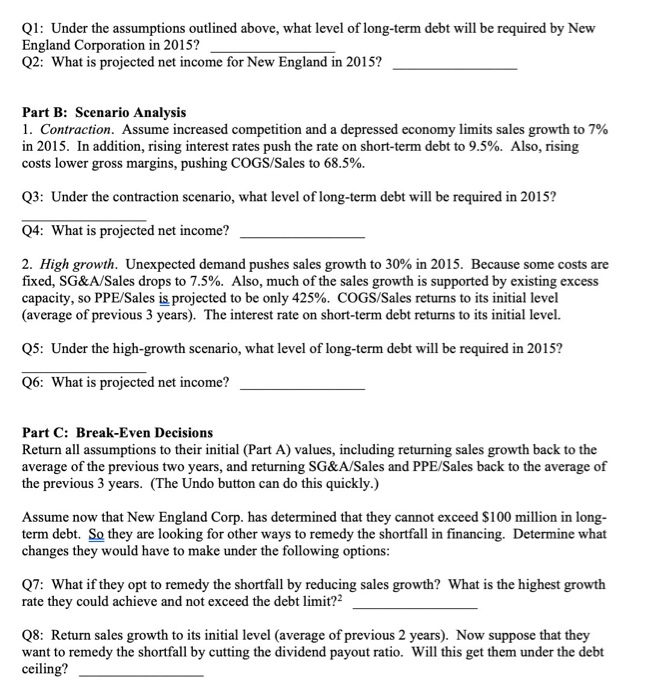
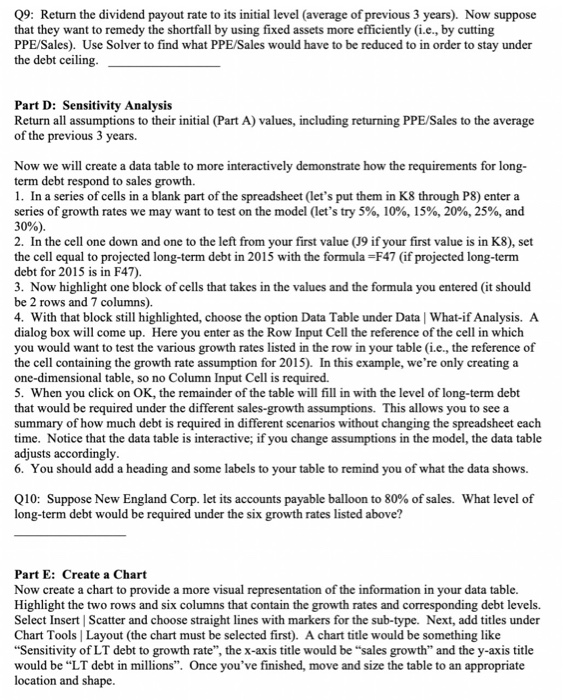
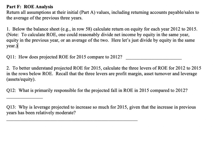
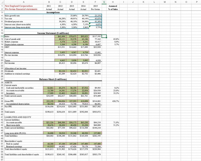
This spreadsheet is set up so that green cells contain numbers and white cells contain formulas. Follow the steps below to prepare pro formas for 2015, assuming that New England Corp. will make up any funding shortfall with long-term debt, and will use any funding surplus to pay down long-term debt (i.e., let long-term debt be the plug figure). 1. As a starting point, assume that sales growth in 2015 will be equal to the average sales growth for 2013 and 2014. Enter the formula for this assumption in the Assumptions section, and then enter the formula for projected sales in 2015. 2. For all financial statement items that would be expected to vary with sales, use the historical average over the past three years of the ratio of that item to sales as a projection of the percentage of sales for 2015. I suggest that you enter these percentages in the column on the right "Assumed % of Sales". (Hint: If you enter your formula correctly in one cell, locking in the appropriate references, then you can simply copy and paste the formula to other cells.) Having this column allows you to return and change the assumption for these items later on. For simplicity, in addition to items that typically vary as a percentage of sales, also assume that depreciation expense, Gross PPE, and short-term debt vary as a percentage of sales. 3. Fill in the 2015 forecast for each item that would be expected to vary with sales. (Again, if you enter the formula correctly, you can copy and paste it to other cells.) 4. Fill in all cells in the 2015 forecast that are just formulas (e.g., pre-tax income is just EBIT - interest expense). 5. Fill in the other items that would not be expected to vary with sales, that is, everything else except for long-term debt. Assumptions for the tax rate, dividend payout rate, and interest rates should be made above in the Assumptions section. For the tax rate and dividend payout rate assume a 2015 projection equal to the average of the previous three years. Assume that interest rates will remain the same as the previous year. Also assume no new equity will be issued in 2015. 6. Fill in long-term debt as the plug figure. This will be the balancing item that makes assets = liabilities + equity, but don't enter the formula as total assets - (total liabilities + equity) or you will get a circular reference (one that can't be remedied with iterative calculation). Instead, you need to make the formula be total assets - current liabilities - total equity. This will balance the balance sheet and not be circular. Q1: Under the assumptions outlined above, what level of long-term debt will be required by New England Corporation in 2015? Q2: What is projected net income for New England in 2015? Part B: Scenario Analysis 1. Contraction. Assume increased competition and a depressed economy limits sales growth to 7% in 2015. In addition, rising interest rates push the rate on short-term debt to 9.5%. Also, rising costs lower gross margins, pushing COGS/Sales to 68.5%. Q3: Under the contraction scenario, what level of long-term debt will be required in 2015? Q4: What is projected net income? 2. High growth. Unexpected demand pushes sales growth to 30% in 2015. Because some costs are fixed, SG&A/Sales drops to 7.5%. Also, much of the sales growth is supported by existing excess capacity, so PPE/Sales is projected to be only 425%. COGS/Sales returns to its initial level (average of previous 3 years). The interest rate on short-term debt returns to its initial level. Q5: Under the high-growth scenario, what level of long-term debt will be required in 2015? Q6: What is projected net income? Part C: Break-Even Decisions Return all assumptions to their initial (Part A) values, including returning sales growth back to the average of the previous two years, and returning SG&A/Sales and PPE/Sales back to the average of the previous 3 years. (The Undo button can do this quickly.) Assume now that New England Corp. has determined that they cannot exceed $100 million in long- term debt. So they are looking for other ways to remedy the shortfall in financing. Determine what changes they would have to make under the following options: Q7: What if they opt to remedy the shortfall by reducing sales growth? What is the highest growth rate they could achieve and not exceed the debt limit?? Q8: Return sales growth to its initial level (average of previous 2 years). Now suppose that they want to remedy the shortfall by cutting the dividend payout ratio. Will this get them under the debt ceiling? Q9: Return the dividend payout rate to its initial level (average of previous 3 years). Now suppose that they want to remedy the shortfall by using fixed assets more efficiently (i.e., by cutting PPE/Sales). Use Solver to find what PPE/Sales would have to be reduced to in order to stay under the debt ceiling. Part D: Sensitivity Analysis Return all assumptions to their initial (Part A) values, including returning PPE/Sales to the average of the previous 3 years. Now we will create a data table to more interactively demonstrate how the requirements for long- term debt respond to sales growth. 1. In a series of cells in a blank part of the spreadsheet (let's put them in K8 through P8) enter a series of growth rates we may want to test on the model (let's try 5%, 10%, 15%, 20%, 25%, and 30%). 2. In the cell one down and one to the left from your first value (J9 if your first value is in K8), set the cell equal to projected long-term debt in 2015 with the formula - F47 (if projected long-term debt for 2015 is in F47). 3. Now highlight one block of cells that takes in the values and the formula you entered (it should be 2 rows and 7 columns). 4. With that block still highlighted, choose the option Data Table under Data | What-if Analysis. A dialog box will come up. Here you enter as the Row Input Cell the reference of the cell in which you would want to test the various growth rates listed in the row in your table (i.e., the reference of the cell containing the growth rate assumption for 2015). In this example, we're only creating a one-dimensional table, so no Column Input Cell is required. 5. When you click on OK, the remainder of the table will fill in with the level of long-term debt that would be required under the different sales-growth assumptions. This allows you to see a summary of how much debt is required in different scenarios without changing the spreadsheet each time. Notice that the data table is interactive; if you change assumptions in the model, the data table adjusts accordingly. 6. You should add a heading and some labels to your table to remind you of what the data shows. Q10: Suppose New England Corp. let its accounts payable balloon to 80% of sales. What level of long-term debt would be required under the six growth rates listed above? Part E: Create a Chart Now create a chart to provide a more visual representation of the information in your data table. Highlight the two rows and six columns that contain the growth rates and corresponding debt levels. Select Insert | Scatter and choose straight lines with markers for the sub-type. Next, add titles under Chart Tools | Layout (the chart must be selected first). A chart title would be something like "Sensitivity of LT debt to growth rate", the x-axis title would be "sales growth" and the y-axis title would be "LT debt in millions". Once you've finished, move and size the table to an appropriate location and shape. Part F: ROE Analysis Return all assumptions at their initial (Part A) values, including returning accounts payable/sales to the average of the previous three years. 1. Below the balance sheet (e.g., in row 58) calculate return on equity for each year 2012 to 2015. (Note: To calculate ROE, one could reasonably divide net income by equity in the same year, equity in the previous year, or an average of the two. Here let's just divide by equity in the same year.) Q11: How does projected ROE for 2015 compare to 2012? 2. To better understand projected ROE for 2015, calculate the three levers of ROE for 2012 to 2015 in the rows below ROE. Recall that the three levers are profit margin, asset turnover and leverage (assets/equity). Q12: What is primarily responsible for the projected fall in ROE in 2015 compared to 2012? Q13: Why is leverage projected to increase so much for 2015, given that the increase in previous years has been relatively moderate? 1 New England Corporation 2 Pro forma financial statements 3 4 Sales growth rate 5 Tax rate 6 Dividend payout rate 7 Interest rate (short-term debt) 8 Interest rate (long-term debt) 9 10 11 Sales 12 Cost of goods sold 13 SG&A expense 14 Depreciation expense 15 EBIT 16 17 Interest expense 18 Pre-tax income 19 20 Taxes 21 Net income 22 23 Allocation of net income: 24 Dividends 25 Addition to retained earnings 26 27 28 ASSETS 29 Current assets 30 Cash and marketable securities 31 Accounts receivable 32 Inventory 33 Total current assets 34 35 Gross PPE 36 Accumulated depreciation 37 Net PPE 38 39 Total assets 40 41 LIABILITIES AND EQUITY 42 Current liabilities 43 Accounts payable 44 Short-term debt 45 Total current liabilities 46 47 Long-term debt (PLUG) 48 Total liabilities 49 B 2011 Actual Assumptions C 2012 Actual 50 Shareholders' equity 51 Paid-in capital 52 Retained earnings 53 Total shareholders equity 54 56 Total liabilities and shareholders' equity 46,28% 39,24% 6,30% 5.30% Income Statement (5 millions) $190,615 5.578 3,268 $13,531 3,455 $10,076 $2,124 $3,289 Balance Sheet (5 millions) D 2013 Actual $62,498 $78,673 $95,023 40,121 52,578 63,186 7,135 8,241 4,298 $14,662 4,663 $5,413 25,88% 20,78% 49,91% 40,14% 48,10% 38,50% 6,50% 7,15% 5.50% 5,96% 4,567 $10,094 E F 2014 2015 Actual Pro forma 5,038 $5,056 $2,432 $2,624 6,106 $17,490 6,724 $10,766 5,092 $5,674 $2.921 $2,752 $6,105 $7.916 $2,861 13,789 17,909 $5,275 14,341 17,276 22,854 22,402 30.991 24.623 $34,559 $42,017 $48,004 $61,761 222,199 284,026 337,593 410,898 66,142 69.410 73,208 79,814 $156,056 $214,616 $263,885 $331,083 $256,634 $311,889 $392,844 $21,326 $48.500 $56,173 $63,250 20.676 28.830 53,258 $42,002 $77,330 $96,622 $116,508 48.930 26.800 30.910 $68,802 $108,240 $131,862 $165,438 60,300 87,100 107.200 147,400 61.513 64.802 67.426 70.178 $121,813 $151,902 $174,626 $217,578 $190,615 $260,142 $306,488 $383,017 23,33% 45,03% 43,30% 6,83% 5,73% $117,193 77,162 10,417 6,687 $22,928 12.002 $10,926 4,920 $6,007 $2,601 $3,406 $9,583 $26,938 $38,969 $75,489 $514,083 $427,582 $503,072 $84,210 $60,000 $144,210 $282,195 147,400 73,584 $220,984 $503,179 G H Assumed % of Sales 65,8% 8,9% 5,7% 8,2% 23,0% 33,3% 438,7% 71,9% 51,2% 1 J K L M N O P