$|$TIA$\_$E$\_$CH$02\_$Technology$\_$Wish$\_$List

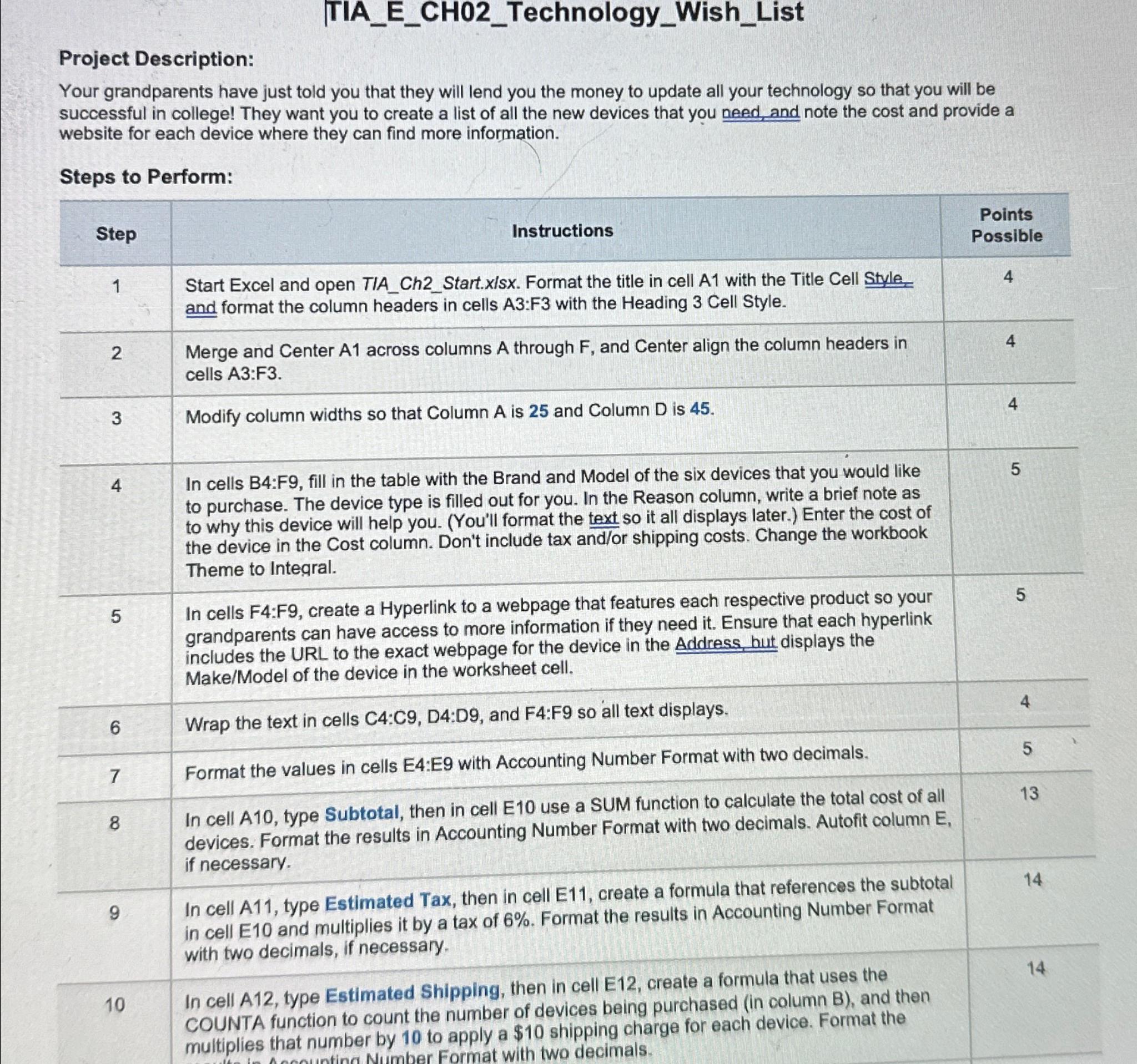
Project Description:

Your grandparents have just told you that they will lend you the money to update all your technology so that you will be successful in college! They want you to create a list of all the new devices that you need, and note the cost and provide a website for each device where they can find more information.

Steps to Perform:

$\backslash$table$[[$Step$,$Instructions,$\backslash$table$[[$Points$],[$Possible$]]],[1,\backslash$table$[[$Start Excel and open TIA$\_$Ch$2\_$Start.xlsx$.$ Format the title in cell A$1$ with the Title Cell Style.$],[$and format the column headers in cells A$3$:F$3$ with the Heading $3$ Cell Style.$]],4],[2,\backslash$table$[[$Merge and Center A$1$ across columns A through F$,$ and Center align the column headers in$],[$cells A$3$:F$3.]],4],[3,$Modify column widths so that Column A is $25$ and Column D is $45.,4],[4,\backslash$table$[[$In cells B$4$:F$9,$ fill in the table with the Brand and Model of the six devices that you would like$],[$to purchase. The device type is filled out for you. In the Reason column, write a brief note as$],[$to why this device will help you. $($You$\text{'}$ll format the text so it all displays later.$)$ Enter the cost of$],[$the device in the Cost column. Don't include tax and$/$or shipping costs. Change the workbook$],[$Theme to Integral.$]],5],[5,\backslash$table$[[$In cells F$4$:F$9,$ create a Hyperlink to a webpage that features each respective product so your$],[$grandparents can have access to more information if they need it$.$ Ensure that each hyperlink$],[$includes the URL to the exact webpage for the device in the Address, hut displays the$],[$Make$/$Model of the device in the worksheet cell.$]],5],[6,$Wrap the text in cells $C4$:$C9,D4$:$D9,$ and $F4$:$F9$ so all text displays.,$4],[7,$Format the values in cells E$4$:E$9$ with Accounting Number Format with two decimals.,$5],[8,\backslash$table$[[$In cell A$10,$ type Subtotal, then in cell E$10$ use a SUM function to calculate the total cost of all$],[$devices$.$ Format the results in Accounting Number Format with two decimals. Autofit column E$,],[$if necessary.$]],13],[9,\backslash$table$[[$In cell A$11,$ type Estimated Tax, then in cell E$11,$ create a formula that references the subtotal$],[$in cell $E10$ and multiplies it by a tax of $6\%.$ Format the results in Accounting Number Format$],[$with two decimals, if necessary.$]],14],[10,\backslash$table$[[$In cell A$12,$ type Estimated Shipping, then in cell E$12,$ create a formula that uses the$],[$COUNTA function to count the number of devices being purchased $($in column B$),$ and then$],[$multiplies that number by $10$ to apply a $$10$ shipping charge for each device. Format the$]],14]]$