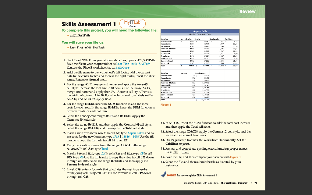
To complete this project, you will need the following flle: - exl01_SA1Path You will save your file as: - Last_First_ex101_SA1Path 1. Start Excel 2016. From your student data files, open exl01_SA1Path. Save the file in your chapter folder as Last_First_exl01_SA1Path Rename the Sheet1 worksheet tab as Path Costs 2. Add the file name to the worksheet's left footer, add the current date to the center footer, and then in the right footer, insert the sheet rame. Return to Normal view. 3. For the range A1:E1, merge and center and apply the Accent 5 cell style. Increase the font size to 18 points. For the range A2:E2, merge and center and apply the 40% - Accent5 cell style. Increase the width of column A to 20. For all oolumn and row labels AA:E4, A5:A14, and A17:C17, apply Bold. 4. For the range E5:E13, insert the SUM function to add the three costs for each row. In the range B14:E14, insert the SUM function to provide totals for each column. 5. Select the nonadjacent ranges B5:E5 and B14:E14. Apply the Currency [0] cell style. rigure 1 6. Select the range B6:E13, and then apply the Comma [0] cell style. 11. In cell C29, insert the SUM function to add the total cost increase, Select the range B14:E14, and then apply the Total cell style. and then apply the Total cell style. 7. Insert a new row above row 7. In cell A7, type Aspen Lakes and as 12. Select the range C20C28, apply the Comma [0] cell style, and then the costs for the new location, type 4763188461498 Use the fill increase the decimal two times. handle to copy the formula in cell E6 to cell E7. 13. Use Page Setup to center the workshect Ilorizontally. Set the 8. Copy the location rames from the range A5:A14 to the range Gridlines to print. A19:A2B. In cell A29, type Total 14. Review and correct any spelling errors, ignoring proper names. 9. In cells B19 and B20, type 03 In cells B21 and B22, type 05 In cell Press Cir J + Home B23, type 06 Use the fill handle to copy the value in cell B23 down 15. Save the file, and then compare your screen with Figure 1. through cell B28. Select the range B19:B2B, and then apply the Percent Style cell style. 16. Close the file, and then submit the file as directed by your 10. In cell C19, enter a formula that calculates the cost increase by instructor. multiplying cell E5 by cell B19. Fill the formula in cell C19 down through cell C2B. BONE! You have completed Shills Assessment 1 Chode ' Warkoozks with Exosi 2010 Microsolt Excel Chapter 1 * 71 To complete this project, you will need the following flle: - exl01_SA1Path You will save your file as: - Last_First_ex101_SA1Path 1. Start Excel 2016. From your student data files, open exl01_SA1Path. Save the file in your chapter folder as Last_First_exl01_SA1Path Rename the Sheet1 worksheet tab as Path Costs 2. Add the file name to the worksheet's left footer, add the current date to the center footer, and then in the right footer, insert the sheet rame. Return to Normal view. 3. For the range A1:E1, merge and center and apply the Accent 5 cell style. Increase the font size to 18 points. For the range A2:E2, merge and center and apply the 40% - Accent5 cell style. Increase the width of column A to 20. For all oolumn and row labels AA:E4, A5:A14, and A17:C17, apply Bold. 4. For the range E5:E13, insert the SUM function to add the three costs for each row. In the range B14:E14, insert the SUM function to provide totals for each column. 5. Select the nonadjacent ranges B5:E5 and B14:E14. Apply the Currency [0] cell style. rigure 1 6. Select the range B6:E13, and then apply the Comma [0] cell style. 11. In cell C29, insert the SUM function to add the total cost increase, Select the range B14:E14, and then apply the Total cell style. and then apply the Total cell style. 7. Insert a new row above row 7. In cell A7, type Aspen Lakes and as 12. Select the range C20C28, apply the Comma [0] cell style, and then the costs for the new location, type 4763188461498 Use the fill increase the decimal two times. handle to copy the formula in cell E6 to cell E7. 13. Use Page Setup to center the workshect Ilorizontally. Set the 8. Copy the location rames from the range A5:A14 to the range Gridlines to print. A19:A2B. In cell A29, type Total 14. Review and correct any spelling errors, ignoring proper names. 9. In cells B19 and B20, type 03 In cells B21 and B22, type 05 In cell Press Cir J + Home B23, type 06 Use the fill handle to copy the value in cell B23 down 15. Save the file, and then compare your screen with Figure 1. through cell B28. Select the range B19:B2B, and then apply the Percent Style cell style. 16. Close the file, and then submit the file as directed by your 10. In cell C19, enter a formula that calculates the cost increase by instructor. multiplying cell E5 by cell B19. Fill the formula in cell C19 down through cell C2B. BONE! You have completed Shills Assessment 1 Chode ' Warkoozks with Exosi 2010 Microsolt Excel Chapter 1 * 71