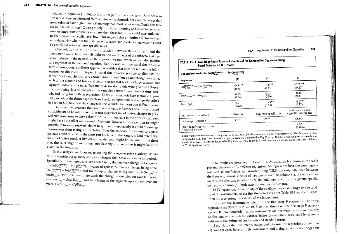
to estimate the regression coefficients in Key RTSLS = on +8 Zi + ... +6 2+ +,Whit ... + +, Write. Concept (10.17) 10.6 10.4 Application to the Demand for Cigarettes 355 where e, is the regression error term. Let F denote the homoskedasticity-only F-statistic testing the hypothesis that of = . . . = 6, = 0. The overidentifying restrictions test statistic is / = mF. Under the null hypothesis that all the instru- The Externalities of Smoking ments are exogenous, then in large samples / is distributed 2 , where m - ke is the "degree of overidentification," that is, the number of instruments minus the moking imposes costs that are not fully borne by after death, the net present value of the per-pack number of endogenous regressors. the smoker, that is, it generates externalities. externalities (the value of the net costs per pack, dis- One economic justification for taxing cigarettes counted to the present) depend on the discount rate. therefore is to "internalize" these externalities. In The studies do not agree on a specific dollar The easiest way to see that you cannot test the exogeneity of the regressors theory, the tax on a pack of cigarettes should equal value of the net externalities. Some suggest the net when the coefficients are exactly identified (m = #) is to consider the case of a sin- the dollar value of the externalities created by smok- externalities, properly discounted, are quite small, gle included endogenous variable (k = 1). If there are two instruments, then you ing that pack. But what, precisely, are the external- less than current taxes. In fact, the most extreme can compute two TSLS estimators, one for each instrument, and you can com- ities of smoking, measured in dollars per pack? estimates suggest that the net externalities are posi- pare them to see if they are close. But if you have only one instrument, then you Several studies have used econometric methods to five, so smoking should be subsidized! Other stud- can compute only one TSLS estimator and you have nothing to compare it to. In estimate the externalities of smoking. The negative ies, which incorporate costs that are probably fact, if the coefficients are exactly identified, so that m = k, then the overidenti- externalities-costs-borne by others include med- important but difficult to quantify (such as caring fying test statistic J is exactly zero. ical costs paid by the government to care for ill smok- for babies who are unhealthy because their moth- ers, health care costs of nonsmokers associated with ers smoke) suggest that externalities might be $1 secondhand smoke, and fires caused by cigarettes. per pack, possibly even more. But all the studies But, from a purely economic point of view, agree that, by tending to die in late middle age, 10.4 Application to the Demand smoking also has positive externalities, or benefits. smokers pay far more in taxes than they ever get for Cigarettes? The biggest benefit of smoking is that smokers tend back in their brief retirement." to pay much more in Social Security (public pen- Our attempt to estimate the elasticity of demand for cigarettes left off with the sion) taxes than they ever get back. There are also 3An early calculation of the externalities of smoking was TSLS estimates summarized in Equation (10.16), in which income was an large savings in nursing home expenditures on the reported by Willard G. Manning et al. (1989). A calcula- included exogenous variable and there were two instruments, the general sales tax very old-smokers tend not to live that long tion suggesting that health care costs would go up if every- one stopped smoking is presented in Barendregt et al. and the cigarette-specific tax. We can now undertake a more careful evaluation Because the negative externalities of smoking occur (1997). Other studies of the externalities of smoking are of these instruments. while the smoker is alive but the positive ones accrue reviewed by Chaloupka and Warner (2000) 2This section assumes knowledge of the material in Sections 8.1 and 8.2 on panel data with T = 2 time periods. As in Section 10.1, it makes sense that the two instruments are relevant because taxes are a big part of the price of cigarettes, and shortly we will look at this empirically. First, however, we focus on the difficult question of whether the two tax variables are plausibly exogenous. The first step in assessing whether an instrument is exogenous is to think through the arguments for why it may or may not be. This requires thinking about what factors account for the error term in the cigarette demand equation and whether these factors are plausibly related to the instruments. Why do some states have higher per capita cigarette consumption than oth- ers? One reason might be variation in incomes across states, but state income is356 CHAPTER 10 Instrumental Variables Regression included in Equation (10.16), so this is not part of the error term. Another rea- son is that there are historical factors influencing demand. For example, states that grow tobacco have higher rates of smoking than most other states, Could this fac- tor be related to taxes? Quite possibly: if tobacco farming and cigarette produc- tion are important industries in a state, then these industries could exert influence to keep cigarette-specific taxes low. This suggests that an omitted factor in ciga- rette demand-whether the state grows tobacco and produces cigarettes-could be correlated with cigarette-specific taxes. One solution to this possible correlation between the error term and the 10.4 Application to the Demand for Cigarettes 357 instrument would be to include information on the size of the tobacco and cig- arette industry in the state; this is the approach we took when we included income as a regressor in the demand equation. But because we have panel data on ciga- TABLE 10.1 Two Stage Least Squares Estimates of the Demand for Cigarettes Using rette consumption, a different approach is available that does not require this infor- Panel Data for 48 U.S. States mation. As discussed in Chapter 8, panel data makes it possible to eliminate the Dependent variable: In(@aggress) - In(@cigaretter) influence of variables that vary across entities (states) but do not change over time, such as the climate and historical circumstances that lead to a large tobacco and Regressor (1) (2) 731 cigarette industry in a state. Two methods for doing this were given in Chapter 0.94+* -1.34** 1.20** B: constructing data on changes in the variables between two different time peri- (0.21 (0.23) (0.20) ods, and using fixed effects regression. To keep the analysis here as simple as pos- 0.53 0.43 0-46 sible, we adopt the former approach and perform regressions of the type described (0.34) (0.30) (0.31) in Section 8.2, based on the changes in the variables between two different years. Intercept 0.21 0.45* * 0.37+ (0.12) The time span between the two different years influences how the estimated (0.13) (0.14) elasticities are to be interpreted. Because cigarettes are addictive, changes in price Both sales tax and will take some time to alter behavior. At first, an increase in the price of cigarettes Instrumental variable(s) Sales tax Cigarette-specific tax cigarette-specific ta might have little effect on demand. Over time, however, the price increase might First-stage F-statistic 33.70 107.20 38.60 contribute to some smokers' desire to quit and, importantly, it could discourage Overidentifying restrictions 4.93 nonsmokers from taking up the habit. Thus the response of demand to a price /-test and p-value (0.026) increase could be small in the short run but large in the long run. Said differently, These regressions were estimated using data for 48 U.5. states (48 observations on the ten-year differences). The data are described or an addictive product like cigarettes, demand might be inelastic in the short in Appendix 10.1. The J-test of overidentifying restrictions is described in Key Concept 10.6 (its p-value is given in parentheses), run, that is, it might have a short-run elasticity near zero, but it might be more and the first-stage F-statistic is described in Key Concept 10.5. Individual coefficients are statistically significant at the *5% level clastic in the long run. or **1% significance level. In this analysis, we focus on estimating the long-run price elasticity. We do this by considering quantity and price changes that occur over ten-year periods. Specifically, in the regressions considered here, the ten-year change in log quan- The results are presented in Table 10.1. As usual, each column in the table city, In(Qometer - In(Qfrances), is regressed against the ten-year change in log price, presents the results of a different regression. All regressions have the same regres- In (prismnewer) - In( Pricenes ), and the ten-year change in log income, In(Inc,) - sors, and all coefficients are estimated using TSLS; the only difference between In(Inc,ma)- Two instruments are used: the change in the sales tax over ten years, the three regressions is the set of instruments used. In column (1), the only instru- Sales Tax, w - Sales Tax,, and the change in the cigarette-specific tax over ten years, CigTax, w - CigTax,, as- ment is the sales tax; in column (2), the only instrument is the cigarette-specific tax; and in column (3), both taxes are used as instruments. In IV regression, the reliability of the coefficient estimates hinge on the valid- ity of the instruments, so the first things to look at in Table 10.1 are the diagnos- tic statistics assessing the validity of the instruments. First, are the instruments relevant? The first-stage F-statistics in the three regressions are 33.7, 107.2, and 88.6, so in all three cases the first-stage F-statistics exceed 10. We conclude that the instruments are not weak, so that we can rely on the standard methods for statistical inference (hypothesis tests, confidence inter- vals) using the estimated coefficients and standard errors. Second, are the instruments exogenous? Because the regressions in columns (1) and (2) each have a single instrument and a single included endogenous358 CHAPTER 10 Instrumental Variables Regression regressor, the coefficients in those regressions are exactly identified. Thus we can- not deploy the J-test in either of those regressions. The regression in column (3). however, is overidentified because there are two instruments and a single included endogenous regressor, so there is one (m - k = 2 -1 = 1) overidentifying restrice tion. The J-statistic is 4.93; this has a 2; distribution, so the 5% critical value is 3.84 (Appendix Table 3) and the null hypothesis that both the instruments are exogenous is rejected at the 5% significance level (this deduction can be made 10.5 Where Do Valid Instruments Come From? 359 directly from the p-value of 0.026, reported in the table). The reason the J-statistic rejects is that the two instruments produce rather The estimate of-0.94 indicates that cigarette consumption is not very inelas- different estimated coefficients. When the only instrument is the sales tax (col- tic: an increase in price of 1% leads to a decrease in consumption of 0.94%. This umn (1)), the estimated price elasticity is -0.94, but when the only instrument is may seem surprising for an addictive product like cigarettes. But remember that the cigarette-specific tax, the estimated price elasticity is -1.34. Recall the basic this elasticity is computed using changes over a ten-year period, so it is a long- idea of the J-statistic: if both instruments are exogenous, then the two TSLS esti- run elasticity. This estimate suggests that increased taxes can make a substantial mators using the individual instruments are consistent and differ from each other dent in cigarette consumption, at least in the long run. only because of random sampling variation. If, however, one of the instruments When the elasticity is estimated using five-year changes from 1985 to 1990, is exogenous and one is not, then the estimator based on the endogenous instru- rather than the ten-year changes reported in Table 10.1, the elasticity (estimated ment is inconsistent, which is detected by the J-statistic. In this application, the with the general sales tax as the instrument) is -0.79; for changes from 1990 to difference between the two estimated price elasticities is sufficiently large that it 1995, the elasticity is -0.68. These estimates suggest that demand is less elastic is unlikely to be the result of pure sampling variation, so the J-statistic rejects the over horizons of five years than ten. This finding of greater price elasticity at null hypothesis that both the instruments are exogenous. longer horizons is consistent with the large body of research on cigarette demand. The J-statistic rejection means that the regression in column (3) is based on Demand elasticity estimates in that literature typically fall in the range -0.3 to invalid instruments (the instrument exogeneity condition fails). What does this -0.5, but these are mainly short-run elasticities; some recent studies suggest that imply about the estimates in columns (1) and (2)? The )-statistic rejection says that the long-run elasticity could be perhaps twice the short-run elasticity.* at least one of the instruments is endogenous, so there are three logical possibili ties: the sales tax is exogenous but the cigarette-specific tax is not, in which case the column (1) regression is reliable; the cigarette-specific tax is exogenous but the sales tax is not, so the column (2) regression is reliable; or neither tax is exoge- 10.5 Where Do Valid Instruments Come From? nous, so neither regression is reliable. The statistical evidence cannot tell us which possibility is correct, so we must use our judgment. In practice the most difficult aspect of IV estimation is finding instruments that We think that the case for the exogeneity of the general sales tax is stronger are both relevant and exogenous. There are two main approaches, which reflect than for the cigarette-specific tax, because the political process can link changes two different perspectives on econometric and statistical modeling. In the cigarette-specific tax to changes in the cigarette market and smoking pol- The first approach is to use economic theory to suggest instruments. For exam- icy. For example, if smoking decreases in a state because it becomes out of fash- ple, the Wrights' understanding of the economics of agricultural markets led them ion, there will be fewer smokers and a weakened lobby against cigarette-specific to look for an instrument that shifted the supply curve but not the demand curve; tax increases, which in turn could lead to higher cigarette-specific taxes. Thus, this in turn led them to consider weather conditions in agricultural regions. One changes in tastes (which are part of u) could be correlated with changes in ciga- area where this approach has been particularly successful is the field of financial rette-specific taxes (the instrument). This suggests discounting the IV estimates economics. Some economic models of investor behavior involve statements about that use the cigarette-only tax as an instrument. This suggests adopting only the how investors forecast, which then imply sets of variables that are uncorrelated with price elasticity estimated using the general sales tax as an instrument, -0.94. the error term. Those models sometimes are nonlinear in the data and in the para- meters, in which case the IV estimators discussed in this chapter cannot be used. An extension of IV methods to nonlinear models, called generalized method of moments estimation, is used instead. Economic theories are, however, abstractions that often do not take into account the nuances and details necessary for analyz- ing a particular data set. Thus this approach does not always work. If you are interested in learning more about the economics of smoking, see Chaloupka and Warner (2000) and Gruber (2001)