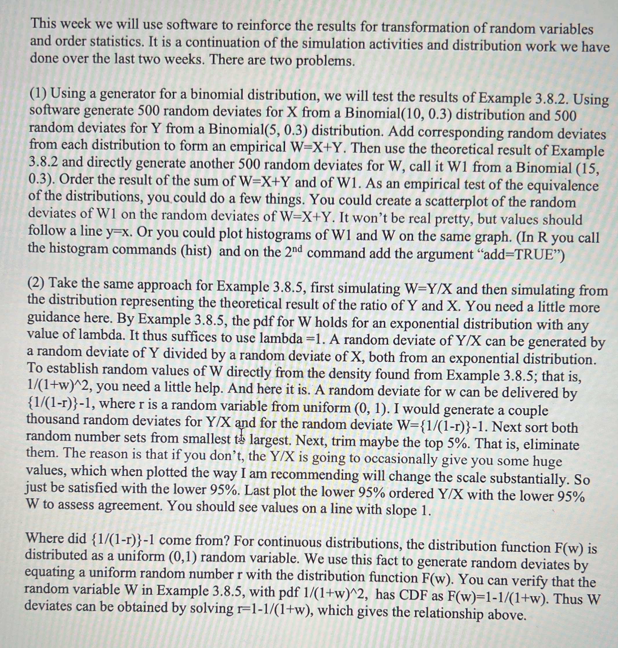
Question: Transforming and combining random variables. Please help with R code examples 3.8.2 and 3.8.5 are from Statistics, Larsen and Marx pages 177 and 180. This
Transforming and combining random variables. Please help with R code examples 3.8.2 and 3.8.5 are from Statistics, Larsen and Marx pages 177 and 180.

This week we will use software to reinforce the results for transformation of random variables and order statistics. It is a continuation of the simulation activities and distribution work we have done over the last two weeks. There are two problems. (1) Using a generator for a binomial distribution, we will test the results of Example 3.8.2. Using software generate 500 random deviates for X from a Binomial(10, 0.3) distribution and 500 random deviates for Y from a Binomial(5, 0.3) distribution. Add corresponding random deviates from each distribution to form an empirical W=X+Y. Then use the theoretical result of Example 3.8.2 and directly generate another 500 random deviates for W, call it WI from a Binomial (15, 0.3). Order the result of the sum of W=X+Y and of W1. As an empirical test of the equivalence of the distributions, you could do a few things. You could create a scatterplot of the random deviates of W1 on the random deviates of W=X+Y. It won't be real pretty, but values should follow a line y x. Or you could plot histograms of WI and W on the same graph. (In R you call the histogram commands (hist) and on the 2nd command add the argument "add=TRUE") (2) Take the same approach for Example 3.8.5, first simulating W=Y/X and then simulating from the distribution representing the theoretical result of the ratio of Y and X. You need a little more guidance here. By Example 3.8.5, the pdf for W holds for an exponential distribution with any value of lambda. It thus suffices to use lambda =1. A random deviate of Y/X can be generated by a random deviate of Y divided by a random deviate of X, both from an exponential distribution. To establish random values of W directly from the density found from Example 3.8.5; that is, 1/(1+w)^2, you need a little help. And here it is. A random deviate for w can be delivered by {1/(1-r)}-1, where r is a random variable from uniform (0, 1). I would generate a couple thousand random deviates for Y/X and for the random deviate W={1/(1-r)}-1. Next sort both random number sets from smallest to largest. Next, trim maybe the top 5%. That is, eliminate them. The reason is that if you don't, the Y/X is going to occasionally give you some huge values, which when plotted the way I am recommending will change the scale substantially. So just be satisfied with the lower 95%. Last plot the lower 95% ordered Y/X with the lower 95% W to assess agreement. You should see values on a line with slope 1. Where did {1/(1-r)}-1 come from? For continuous distributions, the distribution function F(w) is distributed as a uniform (0,1) random variable. We use this fact to generate random deviates by equating a uniform random number r with the distribution function F(w). You can verify that the random variable W in Example 3.8.5, with pdf 1/(1+w) 2, has CDF as F(w)=1-1/(1+w). Thus W deviates can be obtained by solving r=1-1/(1+w), which gives the relationship above
Step by Step Solution
There are 3 Steps involved in it

Get step-by-step solutions from verified subject matter experts


