Tutor, creating your own small excel table to complete this question may be the easiest.

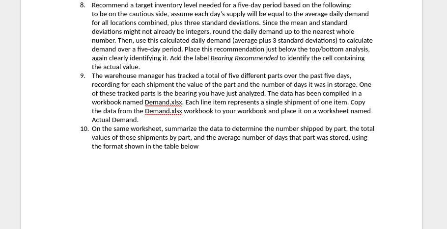
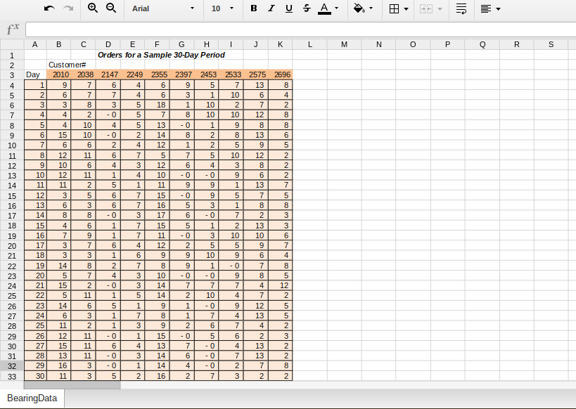
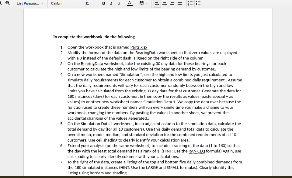
8. Recommend a target inventory level needed for a five-day period based on the following: to be on the cautious side, assume each day's supply will be equal to the average daily demand for all locations combined, plus three standard deviations. Since the mean and standard deviations might not already be integers, round the daily demand up to the nearest whole number. Then, use this calculated daily demand (average plus 3 standard deviations) to calculate demand over a five-day period. Place this recommendation just below the top/bottom analysis, again clearly identifying it. Add the label Bearing Recommended to identify the cell containing the actual value. 9. The warehouse manager has tracked a total of five different parts over the past five days, recording for each shipment the value of the part and the number of days it was in storage. One of these tracked parts is the bearing you have just analyzed. The data has been compiled in a workbook named Demand.xlsx. Each line item represents a single shipment of one item. Copy the data from the Demand.xlsx workbook to your workbook and place it on a worksheet named Actual Demand. 10. On the same worksheet, summarize the data to determine the number shipped by part, the total values of those shipments by part, and the average number of days that part was stored, using the format shown in the table below\f{El List Paraglra... v Calibri 4 r: 4 is. k: 3. 4 E 4 iii |||||| IIIIII |||||| i i To complete the workbook, do the following- '3 Open the workbook that is named Partchlsx Modify the format of the data on the Bearinggata worksheet so that zero values are displayed with a 0 instead of the default dash, aligned on the right side of the column On the BearingData worksheet, take the existing 30 day data for these hearings for each customer to calculate the high and low limits of the bearing demand by customer.. On a new worksheet named "Simulation", use the high and low limits you just calculated to simulate daily requirements for each customer to obtain a combined daily requirement\" Assume that the daily requirements will vary for each customer randomly between the high and low limits you have calculated from the existing 30 day data for that customer. Generate the data for 180 instances (days) for each customer, 5.. then copy the results as values [paste special as values) to another new worksheet names Simulation Data 1. We copy the data over because the function used to create these numbers will run every single time you make a change to your workbook, changing the numbers. By pasting the values in another sheet, we prevent the accidental changing of the values generated. On the Simulation Data 1 worksheet, in an adjacent column to the simulation data, calculate the total demand by day {for all 10 customers]. Use this daily demand total data to calculate the overall mean. mode, median, and standard deviation for the combined requirements of all 10 customers. Use cell shading to clearly identify your calculation area. Extend your analysis (on the same worksheet] to include a ranking of the data (it to 180} so that the day with the least total demand has a rank of 1. (HINT: Use the RANKEE; formula} Again, use cell shading to clearly identify columns with your calculations. To the right of the data, create a listing of the top and bottom ve daily combined demands from the 1510 simulated instances (HINT: Use the LARGE and SWLL formulas}. Clearly identify this listing using borders and shading