Updated comment: This is a complete question rather than a copy of the previous questions (if you compare accurately, I'm sure you'll find this question is completely different from the previous ones)

Before COPYING and PASTING any PREVIOUS ANSWERS, plz read the instruction carefully!

This is a .ipynb file, please fill out the function of basket_option based on the instruction (this is not a big project, just basic stuff):

Code for copy:

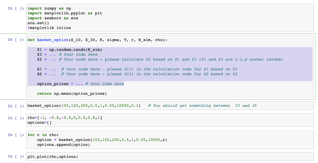
import numpy as np import matplotlib.pyplot as plt import seaborn as sns sns.set() %matplotlib inline

def basket_option(S_10, S_20, K, sigma, T, r, N_sim, rho): Z1 = np.random.randn(N_sim) Z3 = ... # Your code here Z2 = ... # Your code here - please calculate Z2 based on Z1 and Z3 (Z1 and Z3 are i.i.d normal random) S1 = ... # Your code here - please fill in the calculation code for S1 based on Z1 S2 = ... # Your code here - please fill in the calculation code for S2 based on Z2 option_prices = ... # Your Code here return np.mean(option_prices)

basket_option(100,100,200,0.5,1,0.05,10000,0.1) # You should get something between 33 and 35

rho=[-1, -0.8,-0.5,0,0.5,0.8,1] options=[]

for r in rho: option = basket_option(100,100,200,0.5,1,0.05,10000,r) options.append(option)

plt.plot(rho,options)

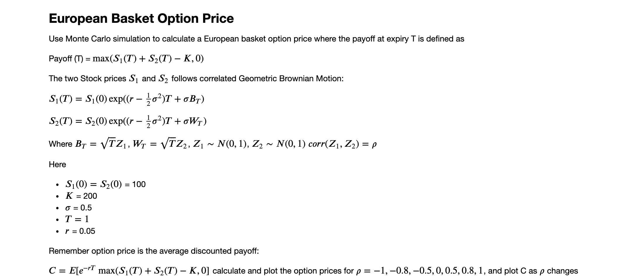
European Basket Option Price Use Monte Carlo simulation to calculate a European basket option price where the payoff at expiry T is defined as Payoff (T) = max(S1(T) + S2(T) K,0) The two Stock prices S and S2 follows correlated Geometric Brownian Motion: Si(T) = Si(0) exp((r 102)T +oBr) S2(T) = S2(0) exp((r 202)T +oWT) Where By = VTZ, W1 = VTZ2, Z, ~ N(0,1), Z2 ~ N(0,1) corr(Z1, Z2) = Here . Si(0) = S2(0) = 100 K = 200 0 = 0.5 T = 1 r = 0.05 Remember option price is the average discounted payoff: C = E[e-rT max(Si(T) + S2(T) K,O] calculate and plot the option prices for p = -1,-0.8,-0.5,0,0.5, 0.8, 1, and plot C as p changes In [ ]: import numpy as np import matplotlib.pyplot as plt import seaborn as sns sns.set() Smatplotlib inline In [ ]: def basket_option(S_10, S_20, K, sigma, T, r, N_sim, rho): z1 = np.random.randn (N_sim) Z3 = ... # Your code here Z2 = # Your code here - please calculate 22 based on 21 and 23 (21 and 23 are i.i.d normal random) S1 = S2 = ... # Your code here - please fill in the calculation code for si based on 21 # Your code here - please fill in the calculation code for s2 based on 22 option_prices = ... * Your Code here return np.mean(option_prices) In [ ]: basket_option (100,100,200,0.5,1,0.05,10000,0.1) # You should get something between 33 and 35 In [ ]: rho=(-1, -0.8,-0.5,0,0.5,0.8,1] options=[] In [ ]: for r in rho: option = basket_option (100,100,200,0.5,1,0.05,10000,1) options.append(option) In [ ]: plt.plot(rho, options) European Basket Option Price Use Monte Carlo simulation to calculate a European basket option price where the payoff at expiry T is defined as Payoff (T) = max(S1(T) + S2(T) K,0) The two Stock prices S and S2 follows correlated Geometric Brownian Motion: Si(T) = Si(0) exp((r 102)T +oBr) S2(T) = S2(0) exp((r 202)T +oWT) Where By = VTZ, W1 = VTZ2, Z, ~ N(0,1), Z2 ~ N(0,1) corr(Z1, Z2) = Here . Si(0) = S2(0) = 100 K = 200 0 = 0.5 T = 1 r = 0.05 Remember option price is the average discounted payoff: C = E[e-rT max(Si(T) + S2(T) K,O] calculate and plot the option prices for p = -1,-0.8,-0.5,0,0.5, 0.8, 1, and plot C as p changes In [ ]: import numpy as np import matplotlib.pyplot as plt import seaborn as sns sns.set() Smatplotlib inline In [ ]: def basket_option(S_10, S_20, K, sigma, T, r, N_sim, rho): z1 = np.random.randn (N_sim) Z3 = ... # Your code here Z2 = # Your code here - please calculate 22 based on 21 and 23 (21 and 23 are i.i.d normal random) S1 = S2 = ... # Your code here - please fill in the calculation code for si based on 21 # Your code here - please fill in the calculation code for s2 based on 22 option_prices = ... * Your Code here return np.mean(option_prices) In [ ]: basket_option (100,100,200,0.5,1,0.05,10000,0.1) # You should get something between 33 and 35 In [ ]: rho=(-1, -0.8,-0.5,0,0.5,0.8,1] options=[] In [ ]: for r in rho: option = basket_option (100,100,200,0.5,1,0.05,10000,1) options.append(option) In [ ]: plt.plot(rho, options)