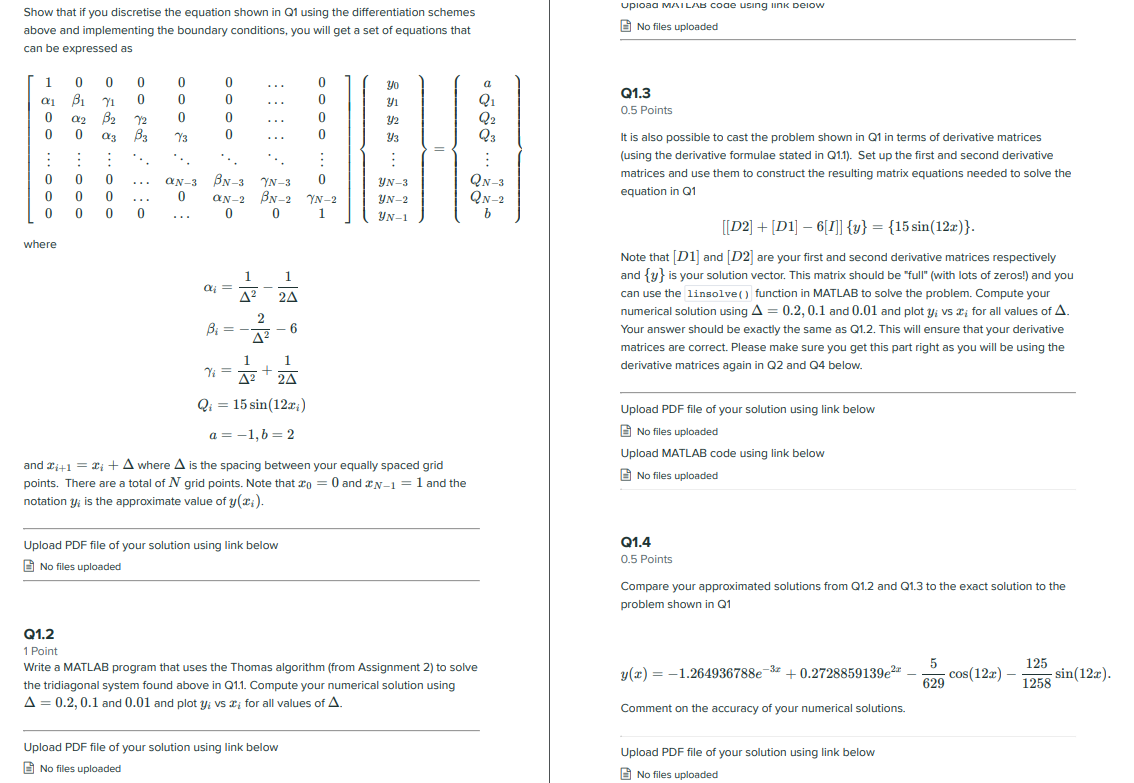
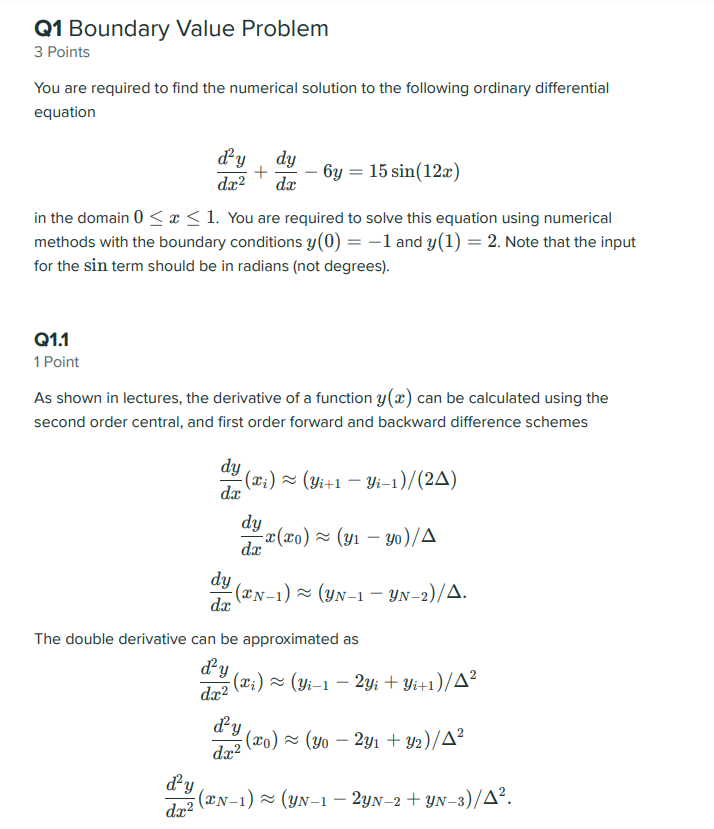
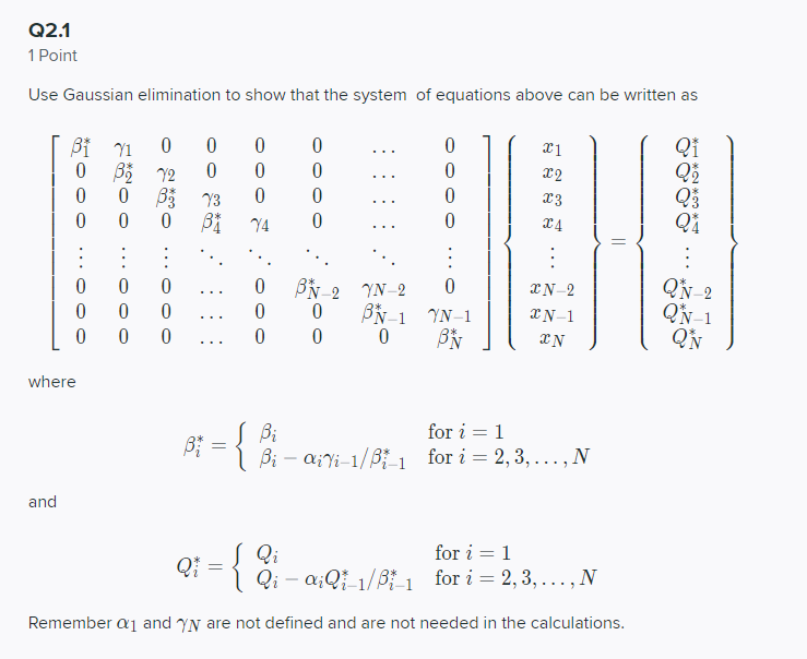
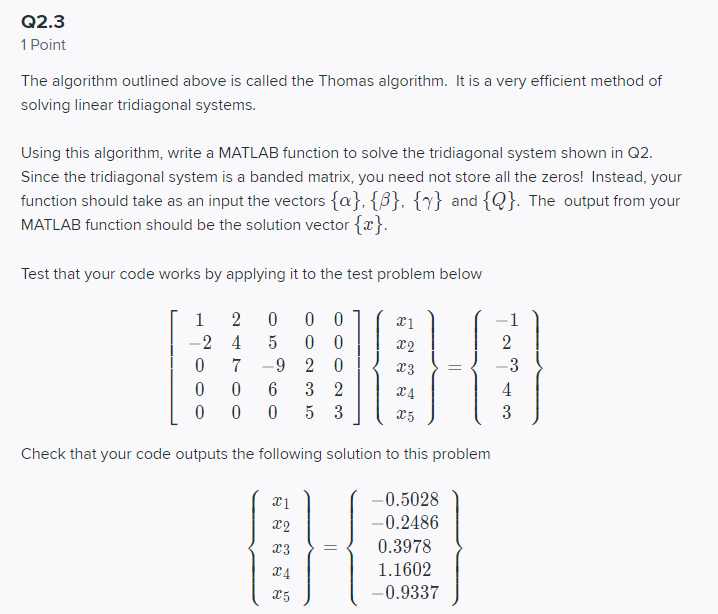
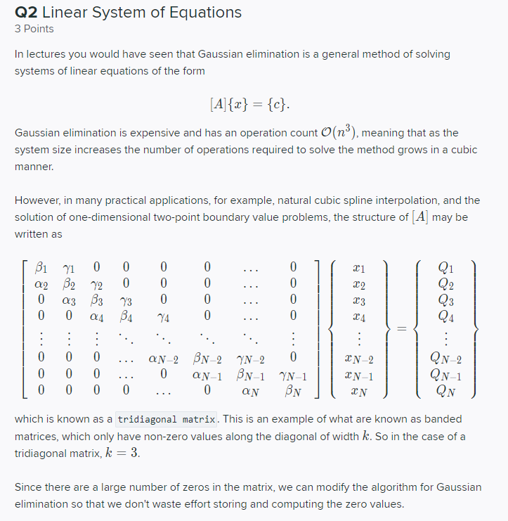
Upload MAILAB code using link below Show that if you discretise the equation shown in @1 using the differentiation schemes above and implementing the boundary conditions, you will get a set of equations that No files uploaded can be expressed as 0 0 0 0 yo a Q1.3 CX1 71 0 . . . Q1 0.5 Points 0 02 B2 72 0 /2 Q2 0 0 B3 0 Q3 It is also possible to cast the problem shown in Q1 in terms of derivative matrices . . . . . . (using the derivative formulae stated in Q1.1). Set up the first and second derivative 10 ... 30 ... DO ... . . . ON-3 BN-3 YN -3 UN-3 QN-3 matrices and use them to construct the resulting matrix equations needed to solve the . . 0 ON-2 BN-2 YN - 2 equation in Q1 yN-2 QN -2 0 0 0 yN-1 b [D2] + [DI] - 6] {y} = {15 sin(12x)}. where Note that [D1] and [ D2] are your first and second derivative matrices respectively 1 and {y} is your solution vector. This matrix should be "full" (with lots of zeros!) and you of = can use the linsolve( ) function in MATLAB to solve the problem. Compute your numerical solution using A = 0.2, 0.1 and 0.01 and plot y: vs ; for all values of A. 2 Bi = - - 6 42 Your answer should be exactly the same as Q1.2. This will ensure that your derivative matrices are correct. Please make sure you get this part right as you will be using the 71 = derivative matrices again in Q2 and Q4 below. 24 Q: = 15 sin(12r;) Upload PDF file of your solution using link below a = -1,b = 2 No files uploaded Upload MATLAB code using link below and Ti+1 = ; + A where A is the spacing between your equally spaced grid points. There are a total of /V grid points. Note that 20 = 0 and CN-1 = 1 and the No files uploaded notation y; is the approximate value of y (I; ). Upload PDF file of your solution using link below Q1.4 0.5 Points No files uploaded Compare your approximated solutions from Q1.2 and Q1.3 to the exact solution to the problem shown in Q1 Q1.2 1 Point Write a MATLAB program that uses the Thomas algorithm (from Assignment 2) to solve 5 125 y(x) = -1.264936788e + 0.2728859139e2 629 - cos(12x) 1258 - sin(12x). the tridiagonal system found above in Q1.1. Compute your numerical solution using A = 0.2, 0.1 and 0.01 and plot y: vs T; for all values of A. Comment on the accuracy of your numerical solutions. Upload PDF file of your solution using link below Upload PDF file of your solution using link below No files uploaded No files uploadedQ1 Boundary Value Problem 3 Points You are required to nd the numerical solution to the following ordinary:r differential equaon d2_y do + -5 = 155i]: 123: in the domain I] E a: i 1. You are required to solve this equation using numerical methods with the ooundanlr conditions y(0) = 1 and y[l) = 2. Note that the input for the sin term should be in radians [not degrees}. Q15 1 Point As shown in lectures. the derivative of a function 3,;(m) can be calculated using the second order central. and rst order forward and backward difference schemes 019 dm [-'-i) * [Elm tied/(23) gem) e [3J1 vol/ d d:($N1 ) m (yer1 - yN2)/ The double derivative can be approximated as a dmEel) ~ [Sit1 - 2s + yeti/a2 a lm? \"r (ya 23:1 + a/2 Q2.1 1 Point Use Gaussian elimination to show that the system of equations above can be written as Qi Bi 0 O 72 Q3 73 . . . QA YA . . . . . O ... YN-2 CN-2 QN-2 O ooo ... . . BN-2 O Ooo BN-1 YN-1 CN-1 QN-1 OO O 0 BN CN QN where Bi for i = 1 = Bi - aivi 1/ Bi_1 for i = 2, 3, . .., N and Qi for 1 = 1 at = ] Qi - aiQt 1/B* 1 for i = 2, 3, . . ., N Remember o1 and y/ are not defined and are not needed in the calculations.Q2.3 1 Point The algorithm outlined above is called the Thomas algorithm. It is a very efficient method of solving linear tridiagonal systems. Using this algorithm, write a MATLAB function to solve the tridiagonal system shown in Q2. Since the tridiagonal system is a banded matrix, you need not store all the zeros! Instead, your function should take as an input the vectors {o} {8}, {} and {@}. The output from your MATLAB function should be the solution vector {x}. Test that your code works by applying it to the test problem below 4 2 0 0 Check that your code outputs the following solution to this problem 0.5028 -0.2486 0.3978 1.1602 C5 0.933702 Linear System of Equations 3 Points In lectures you would have seen that Gaussian elimination is a general method of solving systems of linear equations of the form {Alb} = {C}- Gaussian elimination is expensive and has an operation count 0(n3], meaning that as the system size increases the number of operations required to solve the method grows in a cubic manner. However, in many practical applications, for example, natural cubic spline interpolation, and the solution of onedimensional twopoint boundary value problems, the structure of [A] may be written as ,31 1n 0 [i U i] {i 5131 Q1 De 32 \"r2 0 U U 0 1132 22 0 as 33 T3 0 U U 133 Q3 0 U 0:4 #34 \"F4 0 U 134 _ Q4 0 U U ... cors Ns \"prs 0 DEN2 QNE U U U --- U {IN1 rs1 \"hr1 \"TN1 QN1 U U U U . . . U City y 3N QN which is known as a tridiagonal matrix. This is an example of what are known as banded matrices, which only have nonzero values along the diagonal ofwidth k. So in the case ofa tridiagonal matrix, I: = 3. Since there are a large number of zeros in the matrix, we can modify the algorithm for Gaussian elimination so that we don't waste effort storing and computing the zero values