Use Jupyter Notebook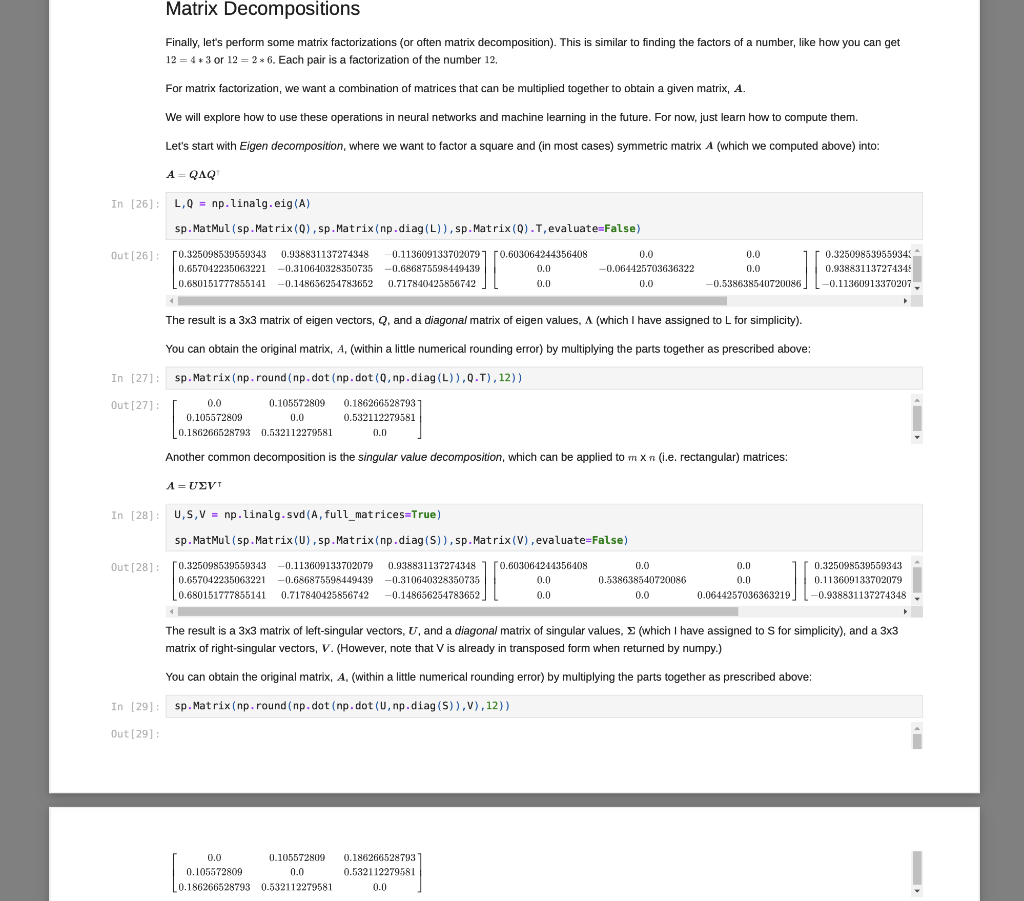

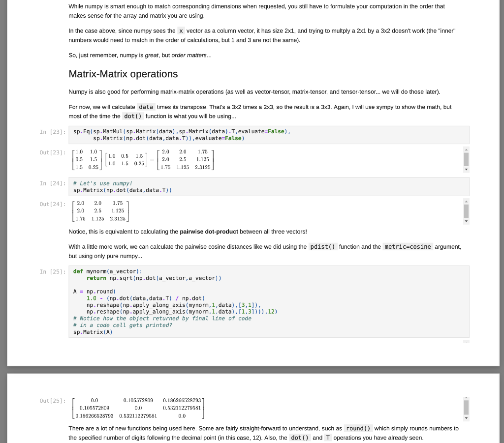
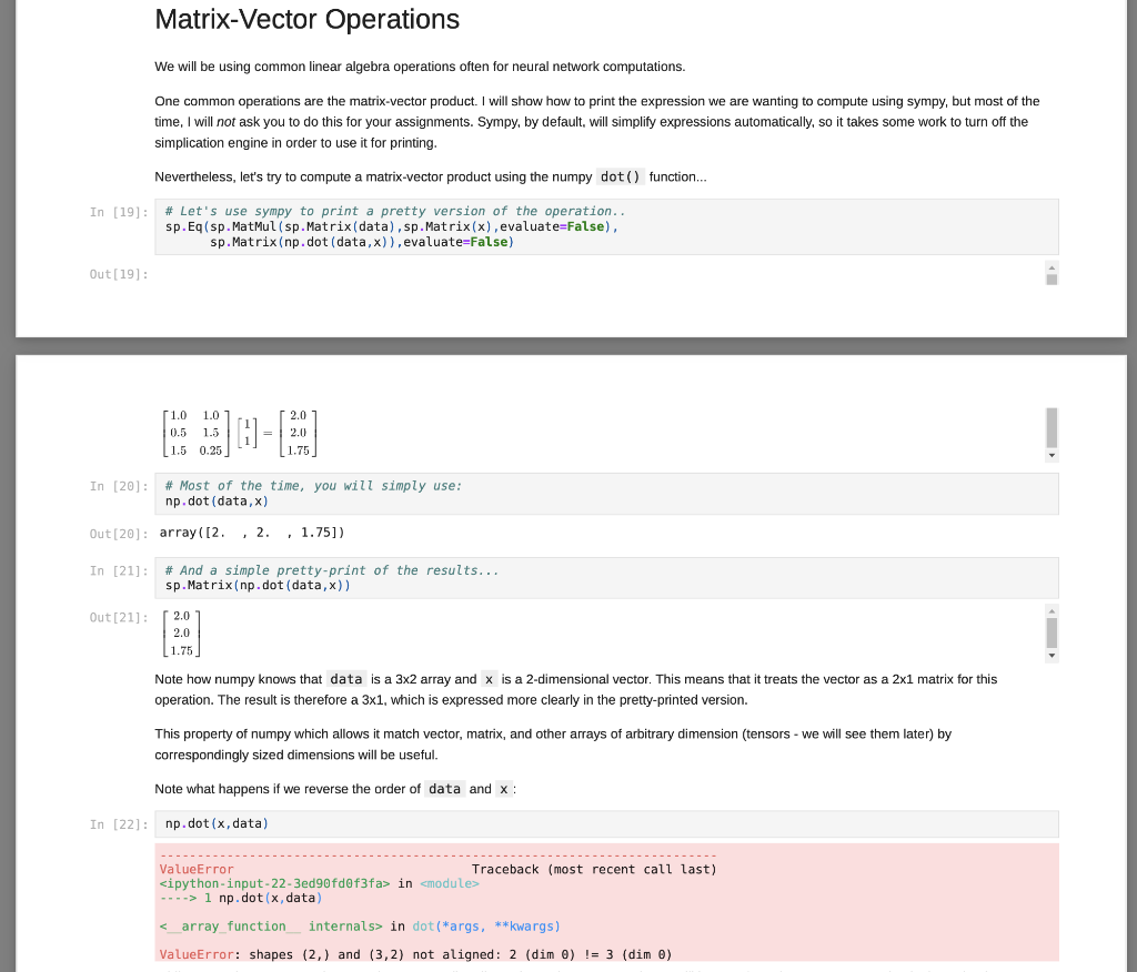
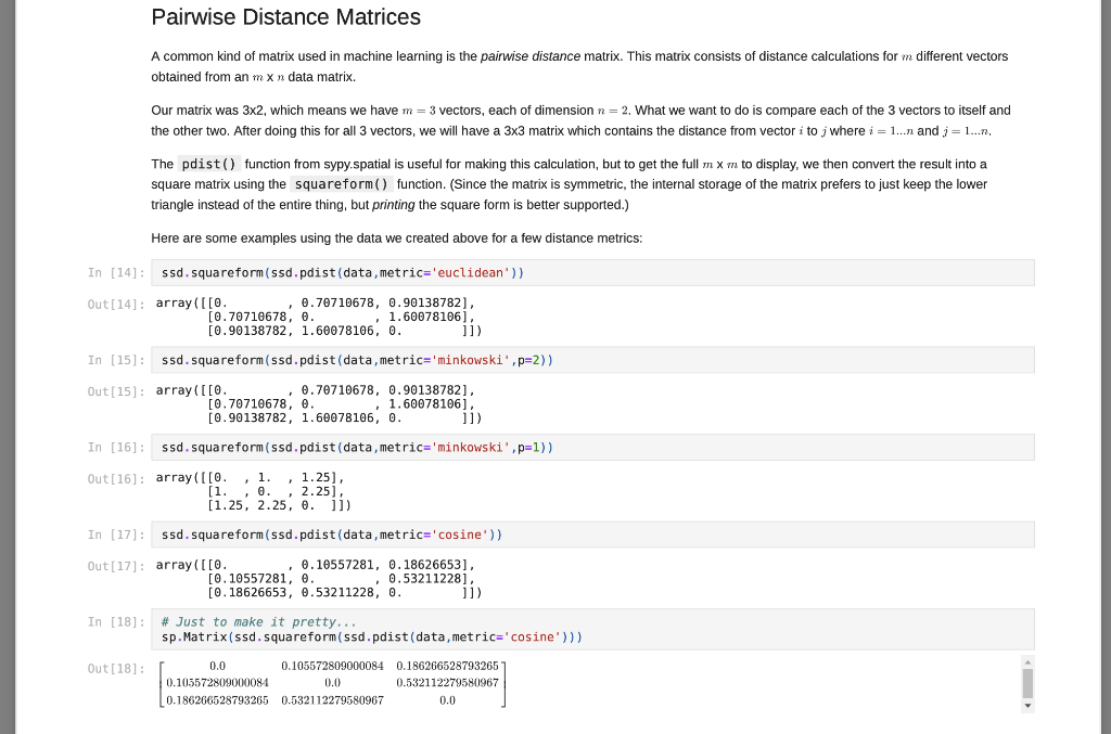
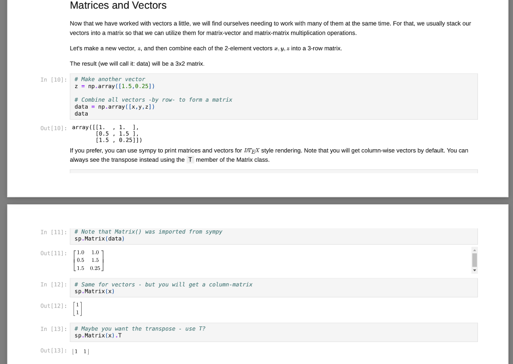
Matrix Decompositions Finally, let's perform some matrix factorizations (or often matrix decomposition). This is similar to finding the factors of a number, like how you can get 12 = 4 * 3 or 12 = 2* 6. Each pair is a factorization of the number 12. For matrix factorization, we want a combination of matrices that can be multiplied together to obtain a given matrix, A. We will explore how to use these operations in neural networks and machine learning in the future. For now, just learn how to compute them. Let's start with Eigen decomposition, where we want to factor a square and (in most cases) symmetric matrix A (which we computed above) into: A-QAQ In (26) L, Q = np. linalg.eig(A) sp.MatMul(sp.Matrix(Q), sp.Matrix(np.diag(L)),sp.Matrix(Q).T, evaluate=False) Out [26] : 50.325098539559343 0.938831137274348 0.657042235063221 -0.310640328350735 0.680151777855141 -0.148636254783652 0.1136091337020797 -0.603064244356408 -0.686875598449439 0.0 0.717840425856742 0.0 0.0 -0.064425703636322 0.0 0.0 0.0 -0.538638540720086 0.325098539559343 0.938831137274345 -0.11360913370207 The result is a 3x3 matrix of eigen vectors, Q, and a diagonal matrix of eigen values, A (which I have assigned to L for simplicity). You can obtain the original matrix, A, (within a little numerical rounding error) by multiplying the parts together as prescribed above: In [27]: sp. Matrix(np.round(np.dot (np.dot(0, np.diag(L)),Q.T), 12)) Out[27] 0.0 0.105572809 0.105572809 0.0 0.186266528793 0.532112279581 0.186266528793 0.532112279581 0.0 Another common decomposition is the singular value decomposition, which can be applied to m X n (i.e. rectangular) matrices: A=USVT In [28]: 0,5, V = np. linalg.svd (A, full_matrices=True) sp.MatMul (sp.Matrix(U), sp. Matrix(np.diag(5)),sp.Matrix(V), evaluate=False) Out [28]: [0.325098539559343 -0.113609133702079 0.938831137271348 0.657042235063221 -0.686875598449439 -0.310640328350735 0.680151777855141 0.717840425856742 -0.148656254783652 0.603061214356408 0.0 0.0 0.0 0.538638540720086 0.0 0.0 0.0 0.0644257036363219 JE 0.325098539559343 0.113609133702079 -0.938831137274348 The result is a 3x3 matrix of left-singular vectors, U, and a diagonal matrix of singular values, (which I have assigned to S for simplicity), and a 3x3 matrix of right-singular vectors, V. (However, note that Vis already in transposed form when returned by numpy.) You can obtain the original matrix, A. (within a little numerical rounding error) by multiplying the parts together as prescribed above: In [29) sp.Matrix(np.round(np.dot (np.dot (U, np.diag(s) ),V),12)) Out [29] : 0.0 0.105572809 0.105572809 0.0 0.186266528793 0.532112279581 0.186266528793 0.532112279581 0.0 While numpy is smart enough to match corresponding dimensions when requested, you still have to formulate your computation in the order that makes sense for the array and matrix you are using. In the case above, since numpy sees the x vector as a column vector, it has size 2x1, and trying to multply a 2x1 by a 3x2 doesn't work (the "inner" numbers would need to match in the order of calculations, but 1 and 3 are not the same). So, just remember, numpy is great, but order matters... Matrix-Matrix operations Numpy is also good for performing matrix-matrix operations (as well as vector-tensor, matrix-tensor, and tensor-tensor... We will do those later). For now, we will calculate data times its transpose. That's a 3x2 times a 2x3, so the result is a 3X3. Again, I will use sympy to show the math, but most of the time the dot() function is what you will be using... In [23]: sp.Eq(sp. Matmul(sp.Matrix(data), sp.Matrix(data). T, evaluate=False), sp.Matrix(np.dot (data, data.T)), evaluate=False) Out [23]: 51.0 1.01 0.5 1.5 1.5 0.25 7. 1.0 0.5 1.51 1.0 1.5 0.25 2.0 2.0 1.75 2.0 2.5 1.125 1.75 1.125 2.3125 In [24]: # Let's use numpy! sp.Matrix(np. dot (data, data. T)) Out [24] : 2.0 2.0 1.75 2.0 2.5 1.125 ( 1.75 1.125 2.3125 Notice, this is equivalent to calculating the pairwise dot-product between all three vectors! With a little more work, we can calculate the pairwise cosine distances like we did using the pdist() function and the metric=cosine argument, but using only pure numpy... In [25]: def mynorm(a vector): return np. sqrt(np.dot(a_vector, a_vector)) A = np. round 1.0 - (np.dot (data, data.T) / np.dot np.reshape (np.apply_along_axis(mynorm, 1, data), [3,1]), np. reshape (np.apply along axis (mynorm, 1, data),[1,3]))),12) # Notice how the object returned by final line of code # in a code cell gets printed? sp.Matrix(A) Out [25]: 0.0 0.105572809 0.105572809 0.0 0.186266528793 0.532112279581 0.186266528793 0.532112279581 0.0 There are a lot of new functions being used here. Some are fairly straight-forward to understand, such as round() which simply rounds numbers to the specified number of digits following the decimal point in this case, 12). Also, the dot() and T operations you have already seen. Matrix-Vector Operations We will be using common linear algebra operations often for neural network computations. One common operations are the matrix-vector product. I will show how to print the expression we are wanting to compute using sympy, but most of the time, I will not ask you to do this for your assignments. Sympy, by default, will simplify expressions automatically, so it takes some work to turn off the simplication engine in order to use it for printing. Nevertheless, let's try to compute a matrix-vector product using the numpy dot() function... In [19]: # Let's use sympy to print a pretty version of the operation.. sp.Eq(sp.MatMul(sp.Matrix(data), sp.Matrix(x), evaluate=False). sp.Matrix(np.dot (data,x)). evaluate=False) Out[19]: 1.0 1.0 0.5 1.5 (1.5 0.25 2.0 = 2.0 | 1.75 In [20]: # Most of the time, you will simply use: np.dot (data,x) Out[20]: array([2. , 2 , 1.75]) In [21]: # And a simple pretty-print of the results... sp.Matrix(np.dot (data,x)) Out [21]: [2.0 2.0 1.75 Note how numpy knows that data is a 3x2 array and x is a 2-dimensional vector. This means that it treats the vector as a 2x1 matrix for this operation. The result therefore a 3x1, which is expressed more clearly in the pretty-printed version. This property of numpy which allows it match vector, matrix, and other arrays of arbitrary dimension (tensors - we will see them later) by correspondingly sized dimensions will be useful. Note what happens if we reverse the order of data and x : In [22]: np.dot (x, data) --------- ValueError Traceback (most recent call last) in ----> 1 np.dot(x, data) in dot(*args, **kwargs) ValueError: shapes (2,) and (3,2) not aligned: 2 (dim ) != 3 (dim ) Pairwise Distance Matrices A common kind of matrix used in machine learning is the pairwise distance matrix. This matrix consists of distance calculations for m different vectors obtained from an m x n data matrix. Our matrix was 3x2, which means we have m = 3 vectors, each of dimension n = 2. What we want to do is compare each of the 3 vectors to itself and the other two. After doing this for all 3 vectors, we will have a 3x3 matrix which contains the distance from vector i to jwhere i=1.... and j = 1...1. The pdist() function from sypy.spatial is useful for making this calculation, but to get the full m X m to display, we then convert the result into a square matrix using the squareform() function. (Since the matrix is symmetric, the internal storage of the matrix prefers to just keep the lower triangle instead of the entire thing, but printing the square form is better supported.) Here are some examples using the data we created above for a few distance metrics: In [14]: ssd.squareform ( ssd.pdist(data,metric='euclidean')) Out[14]: array([[0. 0.70710678, 0.90138782), [0.70710678, 0. , 1.600781061 [0.90138782, 1.60078106, 0. 11) In [15]: ssd.squareform(ssd.pdist (data, metric='minkowski',p=2)) Out[15]: array([[0. , 0.70710678, 0.90138782). [0.70710678, 0. | 1.60078106] 10.90138782, 1.60078106, 0. 11) In [16]: ssd.squareform (Ssd.pdist(data,metric='minkowski',p=1)) Out [16]: array([[0. , 1. , 1.25), [1. , 0.2.25) [1.25, 2.25, 0. jl) In [17]: ssd.squareform(ssd.pdist (data, metric='cosine')) Out[17]: array([[0. 0.10557281, 0.18626653], [0.10557281, 0. 0.53211228] [0.18626653, 0.53211228, 0. 11) In [18]: # Just to make it pretty... sp.Matrix(ssd. squareform( ssd.pdist(data, metric='cosine'))) Out[18]: 0.0 0.105572809000084 0.186266528793265 0.105572809000081 0.0 0.532112279580967 0.186266528793265 0.532112279580967 0.0 Matrices and Vectors Now that we have worked with vectors a little, we will find ourselves needing to work with many of them at the same time. For that, we usually stack our vectors into a matrix so that we can utilize them for matrix-vector and matrix-matrix multiplication operations. Let's make a new vector, z, and then combine each of the 2-element vectors z, y, z into a 3-row matrix. The result (we will call it: data) will be a 3x2 matrix. In [10]: # Make another vector z = np.array([1.5, 0.25]) # Combine all vectors - by row- to form a matrix data = np.array([x,y,z]) data Out[10): array([[1. 1. 1 [0.5, 1.5 L [1.5, 0.25]]) If you prefer, you can use sympy to print matrices and vectors for LTEX style rendering. Note that you will get column-wise vectors by default. You can always see the transpose instead using the T member of the Matrix class. In [11]: x() imported from sympy sp.Matrix(data) Out[11]: 11.01.01 0.5 1.5 1.5 0.25 In [12] : # Same for vectors - but you will get a column-matrix sp.Matrix(x) Out[12]: [1] In [13]: # Maybe you want the transpose - Use T? sp.Matrix(x).T Out[13] : [11] Now that you have had some practice working with vectors and matrices, create a notebook using your new skills that addresses the problems below: 1. Create the vector, c = [5,2,8), and calculate its L2-norm and L1-norm (replace p= 2 with p = 1 in the p-norm equation above). 2. Create another vector, y= (1,3,2), and calculate both the Euclidean and Cosine distances between y and the vector 2. 3. Create and pretty-print the following matrix. 1 2 3 6 A= 7 8 9 10 11 12 13 14 15 4. Multiply A by 2 and y, respectively. That is, calculate Ax and then Ay. Be sure to pretty-print each result. 5. Create the following matrix, B, and then compute the result of AB. 1 2 3 B= 5 6 7 8 9 10 11 12 6. Calculate the pairwise Euclidean distance matrix for the row-vectors in A (pretty-print the result(s)). 7. Calculate the square 3x3 matrix C = BBT (pretty-print the result(s)). 8. Calculate the Eigen Decomposition for C (pretty-print the result(s)). 9. Use the Q and A matrices from Problem 8 to numerically recalculate C (don't forget to pretty-print the result). 10. Calculate the Singular Value Decomposition for C (pretty-print the result(s)). 11. Use the U, 2, and VT matrices from Problem 10 to numerically recalculate C (don't forget to pretty-print the result)