Use the Combination Chart Fashion worksheet to create and format a combination chart exactly as illustrated in
Question:
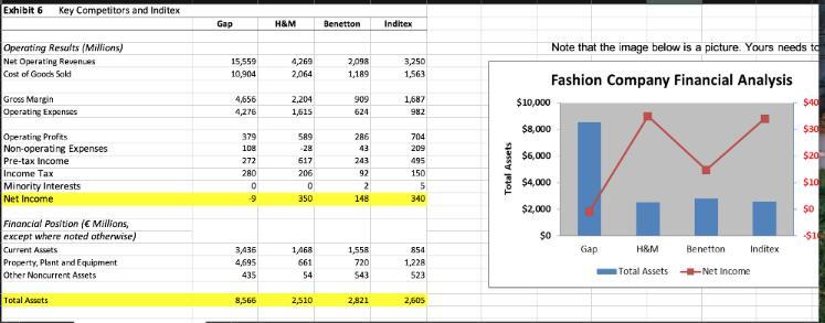
Use the Combination Chart Fashion worksheet to create and format a combination chart exactly as illustrated in the picture provided in the Excel worksheet. The two data series are net income and total assets.
a) First create a 2D column chart of Total Assets. Please enter the series name.
b) Second click the chart area to make it active then click Select Data under the Design tab, and then add the Net Income as a data series. Please enter the series name. Also, add the fashion company names to the horizontal axis by using the Select Data menu - under Horizontal (Category) Axis Labels, hit Edit and highlight the company names.
c) Third, you can plot data on a secondary vertical axis, in this case Net Income. But first change net income to a line graph with markers. In the graph, left click the Net Income series. In the Design tab above, choose Change Chart Type. Find and select the option Line with Markers and select the box for Secondary Axis.
d) Now, format the axis to the desired scale. Right click on the left axis to make it active then select Format Axis. In Axis Options, choose 0, 10,000, and 2,000 for minimum, maximum and major unit respectively. Repeat on the right axis using the appropriate values from the figure.
e) Finish formatting the graph to match the given picture: Legend location, chart title, axis titles, format axis, remove gridlines, and format the plot area. Hint: Under the Design tab and on the left there is a dropdown titled Quick Layout. Under this dropdown look for Layout 3.
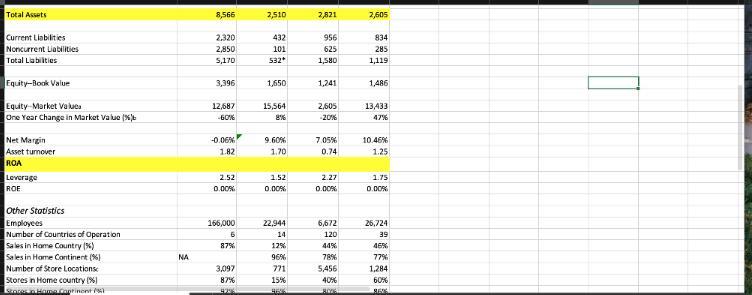
f) Finally, Calculate the Return on Assets (ROA) for each firm and enter the values in B37, C37, D37, and E37 (ROA is defined as the ratio of Net Income to Assets). Format values with a % sign. Why might a manager care about ROA?
Return on Assets (ROA) = Net Income / Total Assets.
Expert Answer: